Reinforcement Learning

With respect to other Machine Learning learning methods, Reinforcement learning doesn’t have a classic supervision, instead we have a reward signal.

Reward

The Reward Signal $r$ is a feedback signal, a scalar, that indicates how well an agent is doing at time $t$.

Reinforcement Learning is based off the Reward Hypothesis which states that all objectives can be described by maximizing the Expected Cumulative Reward.
Training is affected by the decision made during the reward engineering phase, where the reward function is designed.

Reward tells the agent wheter a decision is optimal or not. The Reward function is designed by a system designer, based on measurements of the agent’s performances, ensuring that the learning agent receives the necessary feedback to correct its behaviour.

This can have many problems:

• reward shaping (Ng et al., 1999) sometimes you need to shape the reward signal to one more suitable for learning;
• reward hacking (Skalse et al., 2002) learning agents can exploit reward-specific loopholes to achieve undesired outcomes while still generating high rewards.

Notation

For any integer $n\in \mathbb{N}$, we denote by $[n]$ the set $1,2,...,n$. For any set $S$, $\Delta S$ denotes the set of probability distribution over $S$.
We use $\mathbb{P}(E)$ for the probability of some event $E$, while $\mathbb{E}[X]$ is used to denote the expected value of a random variable $X$. ${\mathbb{E}}_P[\cdot ]$ or similar variations are used to emphasize that the distribution for the expected value is governed by the probability distribution $P\in \Delta (S)$.
Moreover, we will write $X\sim P$ if a random variable $X$ is distributed according to a probability distribution $P$.

Reinforcement Learning, formally

Reinforcement learning is the setting of learning behavior from rewarded interaction with the environment (Sutton & Barto, 2018). It is formalized as a Markov decision process (MDP), which is a model for sequential decision making. It iteratively:

1. Observe its current state;
2. Takes an action taht causes the transition to a new state;
3. Receive a reward that depends on the action effectiveness.

Formally:

• $\mathcal{S}$ is a set of states (the state space);
• $\mathcal{A}$ is a set of actions (the action space);
• $P:\mathcal{S}\times \mathcal{A}\to \Delta (\mathcal{S})$ is a transition function (the transition dynamics);
• $R:\mathcal{S}\times \mathcal{A}\to \mathbb{R}$ is a reward function;
• $d_0\in \Delta (\mathcal{S})$ is a distribution over initial states;
• $\gamma \in [0,1]$ is a discount factor.

The transition function $P$ defines the dynamics of the environemnt: For any state $s$ and action $a$ $P(s^{\prime }|s,a)$ is the probability of reaching $s^{\prime }$ after executing the action $a$ in state $s$.
For a given state and action, the transition probability is conditionally indipendent of all previous states and action (Markov Property).

Instanteneous reward

The value of $R(a,s)\in \mathbb{R}$ provides an immidiate evaluation after performing action $a$ in $s$, which is called instantaneous reward¹.
When both the state space $S$ and the action space $\mathcal{A}$ are finite we call the MDP a tabular MDP.

Return

In an MDP, an $H$-step trajectory $\tau$ is a sequence of $H\in \mathcal{N}\setminus \{0\}$ pairs of state-action ending in a terminal state.
Formally, it is given by $\tau =(s_0,a_0,s_1,a_1,...,s_H)$. Given $t_0\ge 0$ and $H^{\prime }\le H$, we can define a segment $\sigma =(s_{t_0},a_{t_0},s_{t_{0+1}},a_{t_{0+1}},...,s_{H^{\prime }})$ which refers to a continuous sequence of steps within a larger trajectory.
A trajectory $\tau$‘s return $R_t(\tau )$ is the accumulated (and discounted) rewards collected along this trajectory:

$$R_t(\tau )=\sum _{h=0}^{H-1}{\gamma }^{h}R(s_h,a_h)$$

So the return is a projection of future reward by taking a specific series of action-states discounted by a factor that gets exponentially smaller (thus reducing how important are rewards far into the future).

The return is well defined even in the horizon $H$ is infinite as long as $\gamma <1$. If the MDP is a tabular MDP and any trajectory has finite length, i.e. $H$ is necessarily finite, we call the MDP finite, otherwise is infinite.

Policy

A policy specifies how to select actions based on the state the agent is in. Tha can be done either:

• deterministically: in this case we have a mapping $\pi :\mathcal{S}\to \mathcal{A}$ from states to actions.
• stochastically: in this case we have a mapping $\pi :\mathcal{S}\to \Delta (\mathcal{A})$ from states to probability distributions over actions².

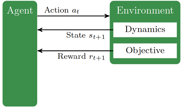
RL basic loop

The basic loop consists in the agent choosing an action $a_t\sim \pi (s_t)$ based on its policy and current state. As a consequence, the environment transition into the new state $s_{t+1}\sim P(s_t,a_t)$, governed by the transition dynamics. The agent observe the new state and the reward $r_{t+1}\sim R(s,a)$ and the cicle starts anew.

In this setting, the RL agent aims at learning a policy that maximizes the expected return:

$$J(\pi )={\mathbb{E}}_{d_0,P,\pi }[R(\tau )]$$

where the expectation is with respect to polici $\pi$, transition function $P$, and initial distribution $d_0$.

Families

To solve this problem there are two different families of RL approaches:

1. Model-based RL

In this family we learn a model (i.e., $P,R$) of the underlying MDP to solve the RL problem.

2. Model-free RL

In this family we try to obtain a good policy without learning an MDP model. This family can also be divided in two sub-families:

2a. Value-based methods

(e.g. DQN)
We aim at learning the $Q$-Function $Q\ast$ of an optimal policy $\pi$ which is defined by

$$Q_{\pi }(s,a)={\mathbb{E}}_{P,\pi }[\sum _{h=0}^{H-1}{\gamma }^{h}R(s_h,a_h)]$$

where $s_0=s$ and $a_0=a$ and in the expectation, $a_h\sim \pi (\cdot |s_h)$ as well as $s_h\sim P(\cdot |s_{h-1},a_{h-1})$ for $h\in [H-1]$. A policy can be designed froma $Q$-function by choosing an action in a greedy manner in each state: $\pi (s)=argma{x}_{a}Q(s,a)$. Note that for deterministic optimal policy $\pi \ast$ it holds that $J(\pi \ast )={\mathbb{E}}_{d_0}[Q\ast (s,\pi \ast (s))]$.
Similar to the action-value function $Q$, we can also define the state-value function:

$$V_{\pi }(s)={\mathbb{E}}_{P,\pi }=[\sum _{h=0}^{H-1}{\gamma }^{h}R(s_h,a_h)|s_0=s]$$

Its value for some state $s$ is the expected return when starting in that state and then always using the policy $\pi$. It is related to the $Q$-Function by means of

$$V_{\pi }(s)={\mathbb{E}}_{a\sim \pi (s)}[Q_{\pi }(s,a)]$$

for any state $s\in S$.

2b. Policy-search methods

This family aims at finding a good policy in some parametrized policy space. The most data-efficient algorithms follow an actor-critic scheme where bot an actor (i.e., a policy) and a critic (i.e., a Q-value function) are learned at the same time (e.g. PPO, TD3, SAC).

In deep RL both the value functions and the policies are approxiamted with neural networks.

RL algorithms can also be further classified as on-policy or off-policy.
In the first case, such as PPO, only the recetly generated transition are used for training. In contrast, in the off-policy algorithms (such as DQN), the agent can be updated with transition non necessarily generated by its current policy.
While on-policy is usually more stable, off-policy enables mode data-efficient learning by reusing samples from a replay buffer taht stores past transitions.

Footnotes

1. It’s possible that in some states the instantaneous reward is zero and the agent receive rewards only in specific states, like the terminal states, for which the transition function in zero. ↩

2. The deterministic case is a special case of the stochastic one, so we assume the latter case. ↩