A Mathematical Framework for Transformers Circuits

The point of Mechanistic Interpretability is taking a Neural Network, and trying to understand the black box. In particular, MI assumes that the model learned human interpretable algorithms with internal coherence, but since it wasn’t trained to expose those algorithms, we need to delve deeper to actually find them out.

An important thing for Mechanistic Interpretability is to understand the motifs for certain outputs. In this paper, Mechanistic Interpretability has been applied to Large Language Models, in particular on Transformers.

The goal of the paper is to prepare a framework on how to do mechanistic interpretability of Transformers.

==The Core Problem in Mechanistic Interpretability is the Curse of Dimensionality==. If you can break down this models into bits that can be interpret independently the problem’s gets manageable.

The Core Framework presented in the paper Skips Over the Multi-layer Perceptron part of the Transformer because it’s hard. And Focuses on Attention-only transformer as a case study, because they’re easier and Attention is the first true new mechanisms in Transformers (kinda not true).

Transformers Overview

The fundamental objective of a transformers is to be a sequence predicting machine. It gets as input a sequence of arbirtrary length, do a bunch of computation in parallel on each elements of the sequence, move information between elements in the sequences using the Attention mechanism, and produce a new element.

Token Embeddings

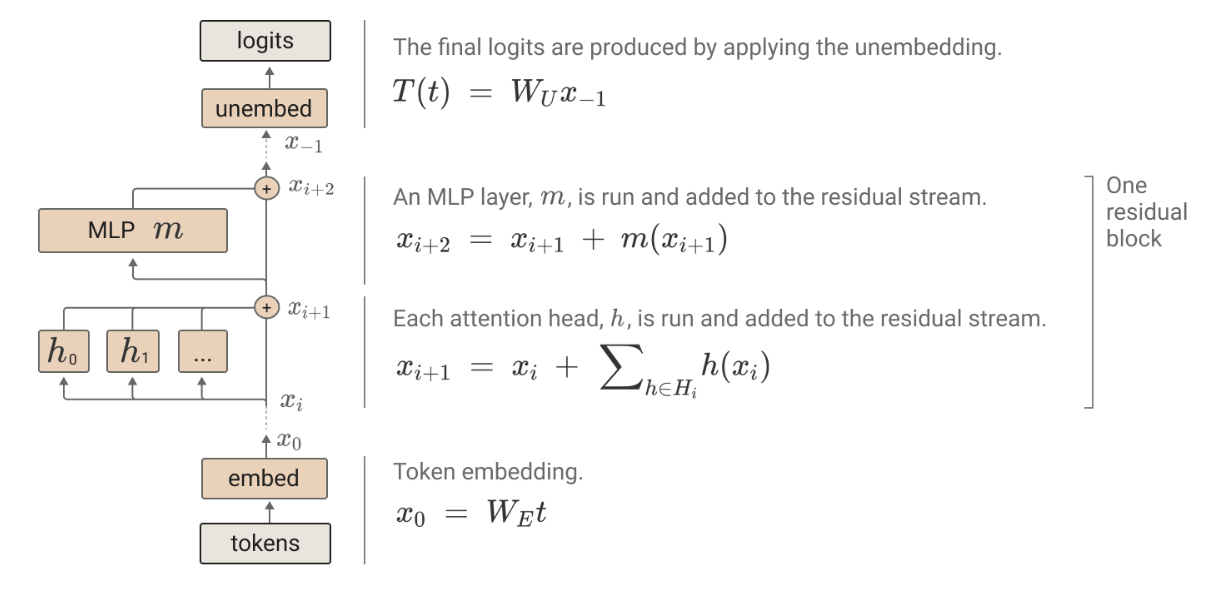
We transform tokens into embeddings by learning a big lookup table $W_E$ where every tokens maps to a vector in this embedding space (if we have a vocab = 50000, and emb_size (or d_model) = 100, we have a lookup table of size 50000 x 100 where every token maps to a vector of size 100)

Positional Encodings

We add to the token embeddings some kind of pattern to represent the position of the token in the sequence. A classic way of doing this is having a matrix $W_{pos}$ of size [d_model x context_size].

Attention Layer

Move information between positions in the sequence.

MLP Layer

Do a bunch of processing for each position in parallel.

Residual stream

Before entering in the Attention Layer or MLP Layer, the input tensor skips around the layer and it’s added back to it’s layer-processed version. It’s the accumulated sum of every output so far.

Unembedding

At the end of the processing we convert this representations in the residual stream which has size [seq_length x d_model]. The unembedding works by applying a linear map to the residual stream which has size [d_model x d_vocab] basically mapping the residual stream onto a matrix of size [seq_length x d_vocab] obtaining the final logits.

This means that for every position in the sequence we have logits of all the vocabulary for the token that should come next.

The paper uses auto-regressive, decoder-only, attention-only Transformers which don’t have MLP Layers.

The Residual Stream

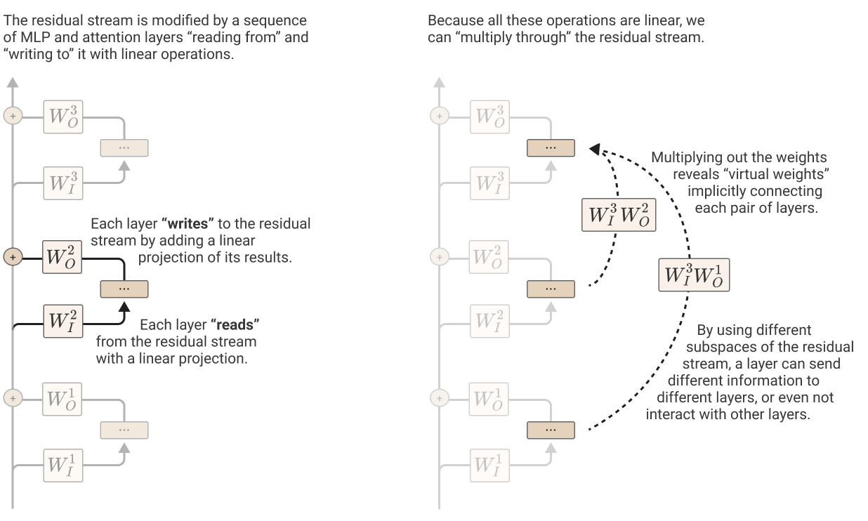
The residual stream in important, it’s like a central object carrying forward all the information of the network and each layer reads it, apply some edits and then put it back (sum edits into it).
The reading and writing of the residual stream is only ever done using linear operations. Mostly addition and linear maps.
This means that you can think as the residual stream as the sum of the output of each layer, and you can decompose the input to any layer, into the sum of a bunch of terms that correspond to different bits of the network.

The residual stream is important because instead of every part needing to go trough all parts of the network the model can choose which layers it wants certain parts to go trough. In practice, most of the computation the model is doing uses just certain layers.

There are two important implication related to the fact that the residual stream is the sum of the outputs of each layer:

1. We expect a lot of the model behavior to be kind of localized. And empirically it seems to be the case: most of the computation done on inputs is done trough a low number of heads and MLPs.
2. The model uses the Residual Streams to achieve composition of different parts of the network (e.g. A head on layer one output something specific of which a head on a different layer focuses on). For any pair of bits of the model they’re free to choose their own encoding. There is no constraint that the “comunication” between L0H0 and L2H5 should be encoded the same as between L0H1 and L3H6. This means that the residual stream is difficult to interpret and empirically this is the case.

Rather than taking the “natural” approach of interpretability of Transformers i.e. the model is a series of tensors and every tensor should be interpretable, this isn’t the case, and the Residual stream itself is completely chaotic, instead we look at which paths are important trough the model.
E.g. there is a path that goes trough embedding, than L0H1, than L2MLP, than unembedding. Hopefully, you can interpret this path and what it does.
Since everything is linear, if you understand the path, you don’t care about understanding the Residual Stream.

A different way to phrase this concept is the idea of a missing privileged basis. A Privileged basis is that if you have a vector space, you gonna need a basis to understand what’s going on (a way to decompose vectors, coefficient to a bunch of fixed axis). There are a bunch of techniques to get a set of vectors and finding a sensible basis, one such technique is Principal Component Analysis (PCA).
If you could a-priori know the right basis, you could go from having a bunch of activations and linear maps to just interpret numbers, and hopefully each number is independently meaningful from the others (often not the case).
There are some parts of the model where we are more likely to find a privileged basis.

Privileged Basis = Knowing a-priori, without looking at any vector, which vector would be meaningful.

---

Complex math stuff: to have a privileged basis you would need something non-linear, but everything that interacts with the Residual Stream is linear. The claim here is that every vector space don’t have a privileged space by default but the residuals and other bits of the models might because they have non-linearity.

---

The goal of this framework is to divide the model into a series of parts some of which are inherently interpretable since they have a privileged basis (tokens, attention patterns, MLP activation and output logits), looking at these and then looking a the linear operations and try to understand those.

Privileged basis shouldn’t be thought as binary but rather at how privileged a basis is.

Virtual Weights

You can think of parts of the model as each layer / component of a layer is reading from the residual stream and writing them out projecting them back to it.
Reading and writing can be pretty misleading, they feel inverse or complementary operation but they are not here. Better words are project for read and embed for write.

Reading or projecting means taking the big residual stream and projecting to something small like the internal dimension of an attention head $h$. Since we are going from big to small, most directions in the residual streams are going to be thrown away, or, in better terms, the model focuses on a subset of meaningful directions: any random vector in the vector space will always going to have non-zero dot product with this directions. So, everything in the Residual Stream, unless it’s literally orthogonal, will have some input to the head, but aligning the thing they read in, with the information they care about, the head can gets mostly the information it cares about. The bit get access to all the information but it can choose to focus on specific things.

Writing or encoding in the other end, means going from small to big, and so it basically means choosing some of the directions of the residual streams and writing the new information onto those, so that future bits of the model can choose to look at those information.

A cool consequence, explained by the idea of virtual weights is that if a bit of the model writes, and another bit read stuff in, we can look at the bit that reads the Residual Stream (knowing that the residual stream is the sum of all previous outputs) than the thing that is being read is the sum of all the previous output of the model, so it’s getting access to all the information. So, you can multiply the writing (embedding) and the reading (projection) weights of two different parts of the model, to get like what is the effective combination of the two things, a crude proxy of what is going on, these are called “Virtual Weights”.

Sub-spaces and Residual Stream Bandwidth

The residual stream is big, but is not that big. In GPT-2 small has width of 768 ($d_{model}=768$), but each MLP layer has width $4d_{model}$. There are 12 MLP Layer all sharing the same Residual Stream. What the paper’s authors think is going on is that the model is compressing more than 768 dimensions in the 768 dimensions of the residual stream, this concept is called Super Position. But, roughly, the idea is that let’s say I have 10k vectors that I want to compress into a vector space of 1000 dimensions, it is impossible to do this with linearly independent set, cause you can only fit in 1000, but if I am willing to accept that my vectors can have dot product that are small but non-zero, I can compress way more vector than a 1000.

Naively, compressing 10k vectors into 1000 dimensions vector space seem kinda fucked. Even if you can get things in, such that any pair of vector has dot product say 0.1, the way you read out information from this thing is that you project onto some direction. If they are orthogonal, this is quite nice, because each feature has a direction and you read out a feature by projecting out onto that feature direction. But if they are not orthogonal, there is interference, and if you got 10k features each of which has non trivial dot product with the feature you care about, than dot product with that feature is going to be completely fucked due to interference. There are two ways that models part from this naive picture:

1. Sparsity. Most feature the model care about are sparse, most of them are not there in any given input. e.g. the feature “Azerbaijan” is sparse, is not there in most texts. This means than rather than thinking about: we’ve got 10k vectors in there, we dot with one, what happens? What actually happens is that we’ve got 10k vectors of which maybe a 100 randomly selected ones are going to be there and then we project onto one. This is a much easier problem with a lot less interference.
2. Correlation. Some feature are gonna be correlated or anti-correlated, if I know that I’ve got the feature “this line of text correspond to a python list variable” it is much less likely that I am gonna have a feature “This line contains the name of an edgy vampire in a romance teen novel”, thus we could have these two feature share a space near each other, because when one is present the other is likely not present, so there is no interference when one is present.

Model can get quite a lot of mileage out of superposition.

Things that makes easier having superposition is only having linear operations, because if you only have linear thing that read and write from a vector space you only have to think about dot products instead of other weird non-linearity.

The model ultimately makes a trade off between representing more features and cleanly read out feature without noise, or interference, and it’s gonna find an optimal trade off which likely isn’t going to be having 0 interference and as many features as there are dimensions.

An important consequence is that the Residual Stream is really hard to interpret.

The Residual Stream is also kind of the model’s memory, and contains all of the outputs of every layer, and the encoded messages sent between layers. This means that we are gonna have messages between like layer 1 and layer 3 and are totally useless for all subsequent layers but it sticks there. The model doesn’t have an automatic way of deleting stuff from the RS.

However, there are some hints about the fact that the models dedicate some of its parameter purely for this purpose, which basically means that some parameters create vectors that are the inverse of certain directions just so that during the dot product those gets cleared out.

Testing for Memory Management

A way to test for these, is to look for MLP neurons looking at the dot product between its input and output weights, and if it’s near -1 it’s deleting information.

In practice, the unembed layer doesn’t really use all the information from the Residual Stream, only parts of it need to be decoded.

How to think about Attention Heads

Conceptually an Attention head $h\in H$ is a bit of the model which works using Attention Pattern: Let’s say we have a sequence abc the head $h$ will learn for each position a probability distribution over that position and previous positions. The head outputs a weighted sum of some information has chosen from previous residual stream weighed by the attention probability on that position, this is done for each token. So, the Attention Matrix is going to be a lower triangle matrix where each row adds up to one. The attention layer output is a concatenation of the output of each head that operates basically independently of the others.

The point of an Attention head is to move information, it is the only point in the Transformer that can move information between position. The Attention pattern tells the head which position to look at, and the head then computes a Value vector (a linear map from the Residual Stream), then we take the Value Vector of each previous position (Source Positions) and take the weighted average by the Attention weights on each previous position (Result vector) and then we multiply this average vector by the output matrix to get a thing that can be added back to the residual stream.

We start with some tensor $x$ which is $[positio{n}_{source}\times d\_model]$ and it’s the Residual Stream.
Then we multiply it with a set of weight $W_{value}^T$ which has dimension $[d\_model\times head\_dim]$.
The Attention weights are of shape $[positio{n}_{destination}\times positio{n}_{source}]$. It’s a square matrix but it’s useful to distinguish the two position type. Then we multiply it by the output weights $W_{output}^T$ which has dimension $[head\_dim\times d\_model]$.
The standard way of chaining this multiplication is $x$ times Value, then times Attention, and finally times the output weights.
But any order is equivalent.

It’s important to distinguish between parameters which are learned and then stored by the model, and activations which are function of a particular input and will vanish when you stop running the model.

Here, $x$ and the Attention Pattern are activations, while the weights are parameters.
N.B.: Attention Pattern are activations because they are generated by the softmaxed dot product of the Query and Key vectors which are obtained from $x$.

So, the weights can be combined into $W_{ov}=W_{output}{W}_{value}$. This tells us that trying to interpret the Value vector is probably fucked because the only thing that determines the product of the head is the product of this two parameter matrices.
The values of the Value vector are probably meaningless, they are simply a middle state.
$W_{ov}$ is of dimension $d\_model\times d\_model$.

So, another fact about this is that the $W_{ov}$ part, is independent of the Attention pattern, you can apply on any order and they touch different parts of $x$.

There are two calculation being done by the Attention head:

1. Where should I get information from? This is done by the Attention pattern which moves you between position.
2. What do I do when I found the positions to move information from? What information I move to my current position? This is done by $W_{ov}$.

These are two related but independent operations done in the heads.