2025.02.04 - Lecture 1

Classical Deep Architecture can be seen as a Bayesian network / using Bayesian formalism. Internal score (logits) are not to be used as a Bayesian estimate.

From Classical Probability to Bayesian Theory

Probability of a given event is the probability of that event w.r.t. of all possible events.
$\Omega$ is the sample space (all that can potentially happen)
$\mathcal{F}=\sigma (\Omega )$ the sigma algebra (Tribù) of events
$P$ the probability measure, which:

• $P(E)\ge 0$, $P(\varnothing )=0$
• $P({\cup }_i^{\text{inf}}{E}_i)={\sum }_i^{\text{inf}}(E_i)$

$\Omega$ is the space of all events
Events $\mathcal{F}$ are all the combination of outcomes you’re interested in.

Mass Probability Function

It is to provide the description of the probability we are interesting in.
The probability mass function of a fair die is:

$$p(x)=\{\begin{array}{ll}& 1/6x=1\\ & 1/6x=2\\ & 1/6x=3\\ & 1/6x=4\\ & 1/6x=5\\ & 1/6x=6\end{array}$$

From Discrete to Continuous distribution

In the continuous case we have to define a mass function density:

$$Pr[a\le X\le b]={\int }_b^{a}fx(x)dx$$

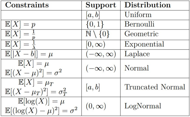
The first part is the interval, the second part is the density. Some famous density function are uniform distribution, the log-normal or the Gaussian.

Shannon Entropy

Entropy is a measure of the amount of knowledge. You can use the Shannon entropy to find the family of distribution for your data.

Definition. Given a discrete random variable $X$, with possible outcomes $e_1,...,e_k$ the Shannon Entropy of $X$ is defined as:

$$\mathcal{H}(X)=\mathbb{E}[-{\log }_b\mathbb{P}(X)]=-\sum _{i=1}^k\mathbb{P}(e_i){\log }_b\mathbb{P}(e_i)$$

Given a random variable $X$ with probability density function $\varphi$ whose support is $\mathcal{S}$ the differential entropy (or continuous entropy) is defined as:

$$\mathcal{H}(X):=-\int {\int }_s\varphi x(x){\log }_b\varphi (x)dx$$

where the base of the logarithm $b$ can be chosen freely. Common choice include $b=2$ or $b=e$.
A maximum entropy probability distribution has entropy that is at least as great as that of all the members of a specified class of probability distributions.

Density in ${\mathbb{R}}^n$

We can look the shadows on each dimensions. Ogni dimensione è una random variable:

$$X_i\sim \mathcal{N}({\mu }_i,{\sigma }_i)$$

This doesn’t let you study co-variance. You need to study simultaneously in every dimension, so, we are going to take a strong assumption, that the directions are independent.

Central Limit Theory

You can ensure that anything becomes a normal distribution by doing a lot of sampling.
Every time you take multiple variables and average it or sum it, you get a gaussian distribution. 1 die has a uniform distribution, if you take 2 and average them you get a gaussian.

Suppose $X_1,X_2,X_3,...$ is a sequence of i.i.d. random variables with $\mathbb{E}[X_i]=\mu$ and $Var[X_i]={\sigma }^2<\infty$. Then, as $n$ approaches infinity, the random variables $\sqrt{n}(\frac{X_1+...+X_n}{n}-\mu )$ converge in distribution to a normal $\mathcal{N}(0,{\sigma }^2)$ .

Random Variable

$(\Omega ,\mathcal{F})$ possibilities and event can be too complex, sometimes intractable.

$$X:(\Omega ,\mathcal{F})\to (E,ϵ)$$

A random variable is a measurable function, which moves the original settings to a easier one, while maintaining some properties of the original space.
e.g.

$$X:\Omega \to \mathbb{R}$$

e.g. If I get 7 by summing two dice I win, otherwise I lose. I don’t care about the space containing all the probabilities, I just want to work with binary possibilities: I win or I lose.

Conditional probability

$P(A\cap B)=P(A|B)P(B)$

The probability of the two events happening at the same time is the probability that A after B happens once B happened.

What is the probability of getting a 2 on a D6, knowing that we got an even number? $\frac{1}{3}$

Conditional Probability works also for continuous r.v.

If A and B are independent then $P(A|B)=P(A)$. e.g. what is the probability of getting a 2 on a D6 knowing that I got a brown die.

Bayesian Formula

$P(A|B)=\frac{P(B|A)P(A)}{P(B)}$

Posterior is $P(A|B)$, $P(B|A)$ is the likelihood, $P(A)$ is the Prior, and $P(B)$ is the evidence.

Likelihood, plauisibility of given a certain outcome when my hypothesis is true.
The prior is what we believe, and likelihood is where we are right.

$$P(\theta |\mathcal{D})=\frac{P(\mathcal{D}|\theta )P(\theta )}{P(\mathcal{D})}$$

Likelihood is the probability of observing the data given the current weights.
Likelihood and loss function are almost the same thing, they are strongly related, we want the model to maximize the likelihood by minimizing the function of the likelihood called loss function.

$$\mathcal{L}(\theta |\{({\mathbf{x}}_i,y_i){\}}_{i=1}^N):=f(\{({\mathbf{x}}_i,y_i{\}}_{i=1}^N|\theta )\underset{i.i.d.}{\underbrace{=}}\prod _{i=1}^{N}f(({\mathbf{x}}_i,y_i)|\theta )$$

The prior in a NN setting is the starting weights.
The posterior is the set of final weights given the input data.

The likelihood is: are my weights given the data?
The second part is the density function, the density of the output.
By definition the likelihood of a given models, given new data, is the “probability” of obtaining those data from the weights of the model.

We assume that each data is independent and identically distributed. And we can rewrite like on the right.

If you have a good prior bayesian learning is very good otherwise bad, you need a lot of data to correct.

Predictive Posterior Distribution

$$p(y|x,\theta )=p(y|X,{\mathcal{M}}_{\theta ,\hat{h}})=p(y|x,\mathcal{D})$$

We are modeling $y$, not $\theta$ like we do in the posterior which are the weights given the dataset. In inference we plug $x$ in the network and we got $y$. We are modeling $y$, the distribution of the predictive posterior.

Artificial Neural Network

Copy Anatomy of a feed forward ANN.

We need a non-linear f because if we don’t have it’s just a linear matrix multiplication and addition and that could be collapsed to a single layer.

The bias is optional.
It acts as a threshold under which the next layer doesn’t change that much. It helps stabilizing.

Recipe of ANN

• A set of hyper-parameters $h$ and trainable parameters.
• Some non linearity.
• An objective function (cost/loss)
• An optimization method
• Sufficient data

The family of neural networks is dense in the function space, any kind of function can model any function.

Feed forward networks with non-polynomial activation functions are dense in the space of continuous functions between two Euclidean spaces, w.r.t. the compact convergence topology.

ANNs training in supervised learning

We need a dataset $D=\{(x,y),\}$ we need to define a measure which compares the quality of the predictions, e.g. MSE.
We also need a way to teach the model how to update weights. We use the gradient, i.e. the best direction of update for the objective function.
Computing the derivative is usually intractable, so we use back-propagation algorithm.

Known Losses

RMSE for regression works really well
Cross Entropy for classification

$$\sum y_i\cdot log(\hat{y}{)}_i$$

The loss is the key of NN.

Reconstruction
we use RMSE