Negative Results for SAEs on Downstream Tasks

from alignment forum.

TL:DR;

• SAEs are missing concepts
• Concepts are represented in noisy ways where e.g. small activations don’t seem interpretable
• Latents can be warped in weird ways like feature absorption
• Seemingly interpretable latents have many false negatives.
• For more issues with SAEs see Section 2.1.2c of Sharkey et al.

These issues should be resolved.
To test if they work well enough they focused on training probes that generalise well out of distribution. We thought that, for sufficiently good SAEs, a sparse probe in SAE latents would be less likely to overfit to minor spurious correlations compared to a dense probe, and thus that being interpretable gave a valuable inductive bias (though are now less confident in this argument). We specifically looked in the context of detecting harmful user intent in the presence of different jailbreaks, and used new jailbreaks as our OOD set.
Sadly, the core results are negative:

1. Dense linear probes perform nearly perfectly, including out of distribution.
2. 1-sparse SAE probes (i.e. using a single SAE latent as a probe) are much worse, failing to fit the training set.
3. k-sparse SAE probes can fit the training set for moderate k (approximately k=20), and successfully generalise to an in-distribution test set, but show distinctly worse performance on the OOD set.
4. Finetuning SAEs on specialised chat data helps, but only closes about half the gap to dense linear probes.
5. Linear probes trained only on the SAE reconstruction are also significantly worse than linear probes on the residual stream OOD, suggesting that SAEs are discarding information relevant to the target concept

Using SAEs for OOD Probing

A natural way to compare SAEs to an established and widely used baseline is by evaluating their ability to identify concepts, such as harmful user intent or the topic of a query directed at a chat model. A common and effective baseline for this task is linear probing, which involves training a linear classifier on labeled examples—both positive and negative—to detect the property of interest.

Since linear probes rely on supervised learning, while SAEs do not, it’s expected that linear probes would perform better within the training distribution. However, when it comes to out-of-distribution generalization, it’s less clear which approach will be more effective.

If SAEs have learned latent representations that align with the model’s actual decision-making features, then using a single SAE latent—or a sparse selection of a few latents—should highlight only the most essential concepts for the task. This could lead to better generalization beyond the training data. In contrast, a dense probe, with its greater capacity, may capture subtler correlations, including spurious ones that do not generalize as well.

To test this, we probe for user prompts that express harmful intent—requests that encourage or enable harm. This task is related to refusal detection, but instead of considering whether the model rejects the request, we label the prompt as ‘harmful’ regardless of whether a jailbreak attempt succeeds in bypassing refusal mechanisms. To introduce distributional shifts, we construct an out-of-distribution (OOD) set by using different datasets and incorporating held-out jailbreak suffixes. This allows us to create hard positives (harmful prompts that don’t appear harmful at first glance) and hard negatives (benign-looking prompts that may seem harmful) for a more rigorous evaluation.

Probing

To conduct probing, we must decide where to apply the probe within the model (both in terms of site and layer) and determine how to aggregate token-level probe results across the context. Since a probe can be applied to any token during the forward pass, the optimal placement isn’t immediately obvious. One approach is to apply the probe at every token position and then aggregate results—such as taking the mean or maximum of the probe’s outputs.

We experimented with two main strategies:

• Max-probing, where we take the maximum activation of a feature along the sequence dimension.
• Fixed-position probing, where the probe is applied at a specific position relative to the first token of the model’s response (e.g., position 0 corresponds to the first response token, -1 to the preceding newline, etc.).

Our findings indicate that max-probing generally performs best. However, probing at position -5—corresponding to the <end_of_turn> token that marks the end of the user’s input—achieves comparable performance. The most reliable results were obtained by probing at layer 20 of Gemma-v2 9B IT.

A study by Bricken et al. found that, for a biology-related task, taking the max of feature activations before training a probe significantly improved the SAE probe’s performance. In our case, however, we observe only a minor advantage over fixed-position probing. ===We hypothesize that this is because information about harmful content naturally accumulates in the <end_of_turn> token, making explicit aggregation less critical.=== This task-specific characteristic may explain differences between our findings and those reported by Anthropic.

Probing with SAEs

We explore two probing methods using SAEs:

1. k-sparse probing on SAE feature activations
   • This assumes that only a single feature (or a small subset) captures the relevant information, reducing the risk of overfitting.
2. Training a linear probe on SAE reconstructions
   • This involves probing the reconstructed activations from SAEs (or a subset of features). While less practical, this helps assess whether the SAE reconstruction retains task-relevant information.

Since our chat SAEs yield consistent results on this task (with a possible slight advantage on the autointerp metric, depending on resampling), we report results using finetuned SAEs, as they allow for faster experimentation.

Linear Probe results

Linear probes on the residual stream perform very well at this task, essentially saturating even on our out of distribution set, indicating information about harmful user intent is present in model activations, obtaining an AUROC of 1.0 on Train and Eval and 0.999 on OOD.

In the plots below, we plot the best single-feature probe of the original GemmaScope SAEs, and a set of SAEs finetuned on chat data (see the finetuning snippet for more details), with the performance of the dense probe shown as a dotted line. =We see that while using finetuned SAEs leads to a significant improvement in single-feature probe performance at this task =- suggesting that these SAEs more closely capture the concept that we care about in a single feature - =they remain below the performance of a dense linear probe, as shown by the dotted line in these plots.=

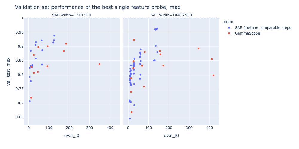
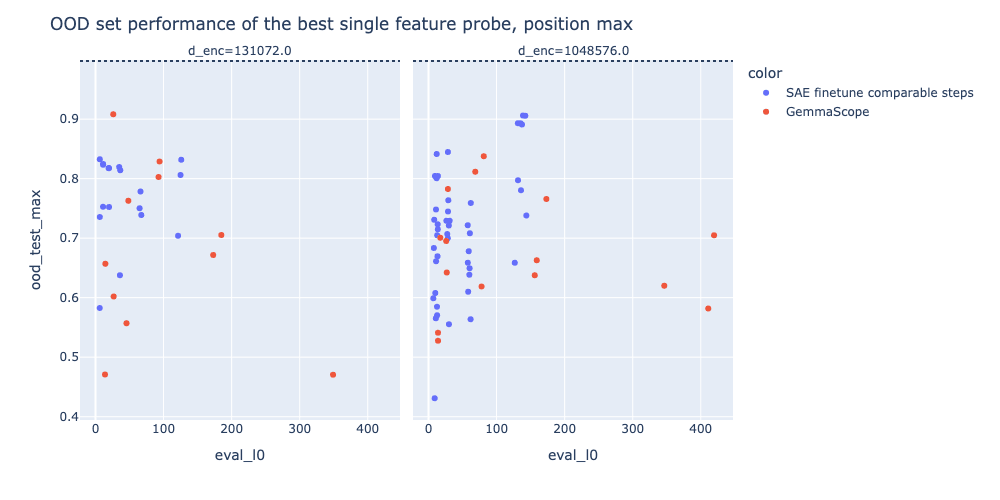
Initially, =we expected that SAE based probes would not outperform linear probes on in-distribution data, but we expected that they might have an advantage out of distribution, especially those based on a single feature or a small number of features, under the hypothesis that SAE features would generalise more robustly out of distribution.= However, we generally find that even on the OOD set, SAE probing does not match the performance of a linear probe, though the best single feature probe from the finetuned model does come close in some cases. We were surprised by the performance and robustness of the linear probe, and this is consistent with probes beating SAEs in OOD settings studied by Kantamneni et al, though we can’t make confident extrapolations about probes vs SAEs in all OOD settings

Interpretability is quite hard to reason clearly about in general. You might have success on a task, but for quite different reasons than you thought, and you might think SAEs should help on a task, but actually your intuition is wrong. To illustrate this, in hindsight, we’re now a lot more confused about whether even an optimal SAE should beat linear probes on OOD generalisation.

Here’s our fuzzy intuition for what’s going on. We have a starting distribution, an OOD distribution, a train set and a val set (from the original distribution) and an OOD test set. There are three kinds of things a probe can learn for predicting the train set:

1. Noise: patterns specific to the train set that do not generalise out of sample, i.e. on the test set. Learning noise gives rise to overfitting.
2. Spurious correlations: patterns that predict the concept in the original distribution (and which are predictive even on the test set) but that do not generalise out of distribution.
3. True signal: patterns that are predictive of the target concept both in-distribution and out-of-distribution.

=Noise is easily ignored given enough data. Indeed, on this task we found that both SAEs and linear probes learn to basically classify perfectly on the test set =(i.e. out of sample, but in-distribution). So the difference in performance between SAEs and linear probes out of distribution comes down to how their respective inductive biases help them to latch on to the true signal versus spurious correlations: it seems that SAE probes do a worse job at this than linear probes. Why is this?

Our initial hypothesis was that sparse SAE probes would provide a better inductive bias, effectively distinguishing the true signal from spurious correlations. This assumption was based on the idea that the concept we aimed to capture—harmful intent—could be expressed as a relatively simple logical function composed of a few fundamental “atomic” concepts. These concepts might include:

• Causal factors (e.g., danger, violence, profanity)
• Correlational signals (e.g., linguistic patterns typical of users attempting harm or jailbreaks)
  We expected that SAEs would naturally assign these atomic concepts to individual latents or small clusters of latents, making it easy for a sparse SAE probe to identify the relevant features while filtering out spurious correlations. However, this did not happen, suggesting several possible issues:

1. Harmful intent may not actually be reducible to a small set of atomic concepts.
   • Even with a perfectly trained SAE—where each latent corresponds precisely to a meaningful concept—it’s possible that the labels in our datasets don’t align with a simple logical expression of just a few such concepts.
   • If true, this raises two possibilities:
     • (a) This could indicate a fundamental limitation of SAEs—we expect them to isolate high-level concepts like harmful intent, and if they fail to do so, this challenges their usefulness.
     • (b) Alternatively, harmful intent might be inherently fuzzy and subjective, depending on human labelers’ interpretations and guidelines. However, if this were the main issue, it would be surprising that linear probes generalize as well as they do.
2. Even if harmful intent is a simple function of a few key concepts, our SAEs may not be learning those concepts cleanly.
   • As a result, sparse SAE probes fail to capture the true signal effectively.
3. SAEs may be missing important components of the true signal.
   • Since SAEs are inherently ** incomplete** , key directions in feature space may be absent from the learned dictionary. This forces the SAE probe to approximate these missing directions using whatever latents it does possess.
4. Spurious correlations may be just as well represented in the SAE dictionary as the true signal.
   • If false spurious signals are encoded as latents just as effectively as meaningful features, then a sparse SAE probe has no reason to prioritize the true signal over misleading correlations.

What This Implies

In practice, we suspect a mix of these factors is at play:

• If (2) and (3) dominate, it suggests we haven’t yet mastered SAE training, but improvement is possible.
• If (1a) holds, it points to deeper limitations of SAEs as a method.
• If (4) is true, SAEs could still be useful for probing—if augmented with techniques to filter out spurious latents. However, we already applied such filtering when cleaning correlations in the dataset, benefiting both SAE probes and dense probes alike.

Overall, this makes it difficult to draw a definitive conclusion from the available data. However, these findings cast doubt on the practical utility of SAEs for probing tasks.