2025.01.22 - Lecture 7

← Lecture 6 · Lecture 8 →

In this lecture (22 January): GENEOs, Group Equivariant Non-Expansive Operators

• Motivation: data and observers, perception pairs
• Elements of the group are isometries (Proposition 41); when $D_G$ is a metric
• Definition of GEO and GENEO and an example
• GENEOs in topological settings, invariant operators
• GENEOs and the natural pseudo-distance
• The space of GENEOs: compactness and convexity
• Comparing data through GENEOs and persistence

Motivation: data and observers

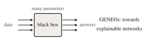
A neural network is a black box with many parameters: data go in, answers come out, and it is hard to explain why. GENEOs aim at explainable networks, built from operators with a precise mathematical meaning and with the symmetries of the problem built in.

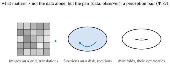
Main point: the data are not so important by themselves; what matters is the pair (data, observer). An observer is described by

• the set $\Phi$ of measurements it can produce (its “instruments”);
• the group $G$ of transformations it considers irrelevant (with respect to which it is equivariant).

This is the perception pair $(\Phi ,G)$ of Lecture 5. Examples: functions on a grid with translations, functions on a ring or disk with rotations, functions on manifolds with their symmetries. Here we stay in the simplicial setting: $\Phi$ is a set of functions on a complex $K$ and $G\subseteq {\mathrm{Iso}}_{\Phi }(K)$.

Elements of the group are isometries

Recall $D_V(x_1,x_2)={\sup }_{\phi \in \Phi }|\phi (x_1)-\phi (x_2)|$ (distance between vertices, as seen by the instruments).

Proposition 41

Every $g\in {\mathrm{Iso}}_{\Phi }(K)$ is an isometry with respect to $D_V$:

$$D_V(g(x_1),g(x_2))=D_V(x_1,x_2).$$

Proof

$$D_V(g(x_1),g(x_2))=\underset{\phi \in \Phi }{\sup }|\phi (g(x_1))-\phi (g(x_2))|=\underset{\phi \in \Phi }{\sup }|(\phi \circ g)(x_1)-(\phi \circ g)(x_2)|.$$

As $\phi$ ranges over $\Phi$, $\phi \circ g$ ranges over all of $\Phi$. It stays in $\Phi$ because $g$ preserves $\Phi$, and it reaches every $\psi \in \Phi$ because $\psi =(\psi \circ g^{-1})\circ g$ with $\psi \circ g^{-1}\in \Phi$. So the map $\phi \mapsto \phi \circ g$ is a bijection of $\Phi$, and the last sup equals ${\sup }_{\psi \in \Phi }|\psi (x_1)-\psi (x_2)|=D_V(x_1,x_2)$. $■$

Using only $\phi \circ g\in \Phi$ we would get just "$\le$". This is why ${\mathrm{Iso}}_{\Phi }(K)$ also requires $\phi \circ g^{-1}\in \Phi$.

Recall also

$$D_G(g_1,g_2)=\underset{\phi \in \Phi }{\sup }\Vert \phi \circ g_1-\phi \circ g_2{\Vert }_{\infty }:$$

two transformations are different only if some measurement reveals a difference between them, and then that is good enough to separate them.

Proposition – If $D_V$ is a metric, then $D_G$ is a metric

Exchanging the two sups,

$$D_G(g_1,g_2)=\underset{\phi \in \Phi }{\sup }\underset{v}{\max }|\phi (g_1(v))-\phi (g_2(v))|=\underset{v}{\max }{D}_V(g_1(v),g_2(v)).$$

If $D_G(g_1,g_2)=0$, then $D_V(g_1(v),g_2(v))=0$ for every vertex $v$, so $g_1(v)=g_2(v)$ (since $D_V$ is a metric), and therefore $g_1=g_2$: an isomorphism is determined by what it does on the vertices.

GEOs and GENEOs

Let $(\Phi ,G)$ and $(\Psi ,H)$ be two perception pairs. The functions in $\Phi$ and $\Psi$ can live on different complexes and the groups can be different.

Definition – GEO (Group Equivariant Operator)

A pair $(F,T)$ with

1. $F:\Phi \to \Psi$,
2. $T:G\to H$ a group homomorphism ($T(g_1{g}_2)=T(g_1)T(g_2)$),

is a GEO from $(\Phi ,G)$ to $(\Psi ,H)$ if

$$F(\phi \circ g)=F(\phi )\circ T(g)\forall \phi \in \Phi ,\forall g\in G.$$

Transforming the input by $g$ and then applying $F$ is the same as applying $F$ and then transforming the output by the corresponding $T(g)$.

Typo in the handwritten notes

The notes write $F(\phi \circ g)=F(\phi )\cdot F(g)$; the correct right-hand side is $F(\phi )\circ T(g)$. $F$ acts on functions, not on group elements.

Definition – GENEO

A GEO $(F,T)$ is a GENEO (Group Equivariant Non-Expansive Operator) if $F$ is non-expansive:

$$D_{\Psi }(F({\phi }_1),F({\phi }_2))\le D_{\Phi }({\phi }_1,{\phi }_2),\text{i.e.}\Vert F({\phi }_1)-F({\phi }_2){\Vert }_{\infty }\le \Vert {\phi }_1-{\phi }_2{\Vert }_{\infty }.$$

The images $F({\phi }_1),F({\phi }_2)$ are at most as far apart as ${\phi }_1,{\phi }_2$.

Example: from the hexagon to the triangle

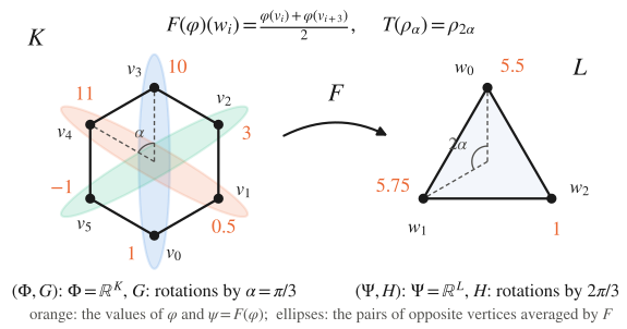
• $(\Phi ,G)$: $K$ is the hexagon with vertices $v_0,\dots ,v_5$, $\Phi ={\mathbb{R}}^K$ (all functions on its vertices), $G$ = the rotations ${\rho }_{\alpha }$ by multiples of $\alpha =\pi /3$, with ${\rho }_{\pi /3}(v_j)=v_{j+1}$ (indices mod 6).
• $(\Psi ,H)$: $L$ is the triangle with vertices $w_0,w_1,w_2$, $\Psi ={\mathbb{R}}^L$, $H$ = the rotations by multiples of $2\pi /3$, with ${\rho }_{2\pi /3}(w_i)=w_{i+1}$ (indices mod 3).
• $T:G\to H$, $T({\rho }_{\alpha })={\rho }_{2\alpha }$: rotating the hexagon by $\pi /3$ corresponds to rotating the triangle by $2\pi /3$. It is a homomorphism, since ${\rho }_{\alpha +\beta }\mapsto {\rho }_{2\alpha +2\beta }={\rho }_{2\alpha }\circ {\rho }_{2\beta }$. It is not injective: the half-turn ${\rho }_{\pi }$ goes to ${\rho }_{2\pi }=\mathrm{id}$.
• $F(\phi )=\psi$ with

$$\psi (w_i)=\frac{\phi (v_i)+\phi (v_{i+3})}{2},i=0,1,2,$$

the average of each pair of opposite vertices of the hexagon (the coloured ellipses).

With the values in the picture, $\phi (v_0,\dots ,v_5)=(1,0.5,3,10,11,-1)$, we get $\psi (w_0)=\frac{1+10}{2}=5.5$, $\psi (w_1)=\frac{0.5+11}{2}=5.75$, $\psi (w_2)=\frac{3-1}{2}=1$.

Proof that $(F,T)$ is a GENEO

Equivariance. Let $\rho ={\rho }_{\pi /3}$, so $(\phi \circ \rho )(v_j)=\phi (v_{j+1})$ and $T(\rho )={\rho }_{2\pi /3}$. For every $i$:

$$F(\phi \circ \rho )(w_i)=\frac{\phi (v_{i+1})+\phi (v_{i+4})}{2},(F(\phi )\circ {\rho }_{2\pi /3})(w_i)=F(\phi )(w_{i+1})=\frac{\phi (v_{i+1})+\phi (v_{i+4})}{2}.$$

For $i=2$, $w_{i+1}=w_0$ gives $\frac{\phi (v_0)+\phi (v_3)}{2}$, the same as $\frac{\phi (v_3)+\phi (v_6)}{2}$ since $v_6=v_0$. In the notes: $F(\phi \circ {\rho }_{\pi /3})(w_0)=\frac{\phi (v_1)+\phi (v_4)}{2}=F(\phi )(w_1)=(F(\phi )\circ {\rho }_{2\pi /3})(w_0)$, and the same holds at every point. Both sides are compatible with composition, so the identity extends from the generator $\rho$ to all of $G$.

Non-expansivity.

$$|F({\phi }_1)(w_i)-F({\phi }_2)(w_i)|\le \frac{1}{2}|{\phi }_1(v_i)-{\phi }_2(v_i)|+\frac{1}{2}|{\phi }_1(v_{i+3})-{\phi }_2(v_{i+3})|\le \Vert {\phi }_1-{\phi }_2{\Vert }_{\infty }.$$

GENEOs in topological settings, invariance

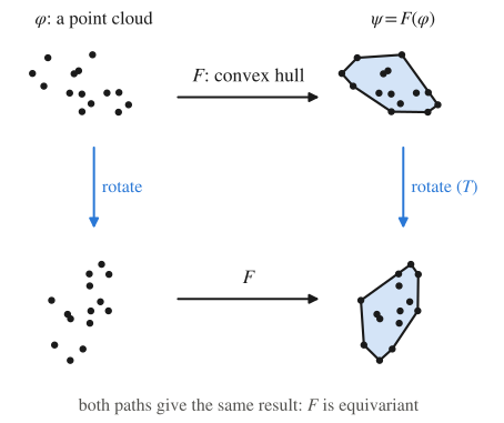
Example: $\phi$ is a point cloud and $F$ takes its convex hull. Rotating the cloud and then taking the hull gives the same result as taking the hull and then rotating it: $F$ is equivariant with respect to rotations, with $T$ the identity. It is also non-expansive for the Hausdorff distance between sets.

Invariance is a special case of equivariance

If we want to model invariance instead of equivariance, it suffices to take the trivial homomorphism $T(g)={\mathrm{id}}_Y$ for all $g$ (${\mathrm{id}}_Y$ is the identity of the domain $Y$ of the functions in $\Psi$). Then

$$F(\phi \circ g)=F(\phi )\circ T(g)=F(\phi )\circ {\mathrm{id}}_Y=F(\phi ):$$

the output does not change at all when the input is transformed. Persistence ($\phi \mapsto \mathrm{Dgm}(\phi )$) is an invariant, non-expansive operator of this kind: the persistence diagram is a trivial GENEO.

GENEOs and the natural pseudo-distance

Proposition

If $(F,T):(\Phi ,G)\to (\Psi ,H)$ is a GENEO (so $D_{\Psi }(F({\phi }_1),F({\phi }_2))\le D_{\Phi }({\phi }_1,{\phi }_2)$), then

$$d_H(F({\phi }_1),F({\phi }_2))\le d_G({\phi }_1,{\phi }_2).$$

GENEOs are non-expansive also with respect to the natural pseudo-distances.

Proof

$$\begin{array}{rl}{d}_H(F({\phi }_1),F({\phi }_2))& =\underset{h\in H}{\min }\Vert F({\phi }_1)-F({\phi }_2)\circ h{\Vert }_{\infty }\le \underset{g\in G}{\min }\Vert F({\phi }_1)-F({\phi }_2)\circ T(g){\Vert }_{\infty }\\ & =\underset{g\in G}{\min }\Vert F({\phi }_1)-F({\phi }_2\circ g){\Vert }_{\infty }\le \underset{g\in G}{\min }\Vert {\phi }_1-{\phi }_2\circ g{\Vert }_{\infty }=d_G({\phi }_1,{\phi }_2).\end{array}$$

The first inequality holds because $T(G)\subseteq H$ (fewer candidates), the equality is equivariance, the last inequality is non-expansivity. $■$

The space of GENEOs: compactness and convexity

Fix $T:G\to H$ and let ${\mathcal{F}}_T^{\mathrm{all}}$ be the set of all maps $F$ such that $(F,T)$ is a GENEO from $(\Phi ,G)$ to $(\Psi ,H)$. We measure distances between operators by

$$D_{\mathrm{GENEO}}(F_1,F_2)=\underset{\phi \in \Phi }{\sup }{D}_{\Psi }(F_1(\phi ),F_2(\phi ))=\underset{\phi \in \Phi }{\sup }\Vert F_1(\phi )-F_2(\phi ){\Vert }_{\infty }.$$

Theorem – Compactness

If $\Phi$ and $\Psi$ are compact, then ${\mathcal{F}}_T^{\mathrm{all}}$ is compact with respect to $D_{\mathrm{GENEO}}$.

When input and output are compact, the space of “agents” (observers) is compact too. In practice, for every $\epsilon >0$ finitely many GENEOs approximate all of them within $\epsilon$, so the space can be explored and sampled. Compare with neural networks, whose parameter spaces are not compact. (The proof is a diagonal argument; see Frosini et al., Theorem 12.)

Theorem – Combinations of GENEOs

Let $(F_1,T),\dots ,(F_n,T)$ be GENEOs from $(\Phi ,G)$ to $(\Psi ,H)$ and $(a_1,\dots ,a_n)\in {\mathbb{R}}^n$ with ${\sum }_i|a_i|\le 1$. If $F_{\Sigma }:={\sum }_i{a}_i{F}_i$ maps $\Phi$ into $\Psi$, then $(F_{\Sigma },T)$ is a GENEO.

Proof

Equivariance:

$$F_{\Sigma }(\phi \circ g)=\sum _i{a}_i{F}_i(\phi \circ g)=\sum _i{a}_i(F_i(\phi )\circ T(g))=(\sum _i{a}_i{F}_i(\phi ))\circ T(g)=F_{\Sigma }(\phi )\circ T(g).$$

Non-expansivity:

$$\begin{array}{rl}\Vert F_{\Sigma }({\phi }_1)-F_{\Sigma }({\phi }_2){\Vert }_{\infty }& =\Vert \sum _i{a}_i(F_i({\phi }_1)-F_i({\phi }_2)){\Vert }_{\infty }\le \sum _i|a_i|\Vert F_i({\phi }_1)-F_i({\phi }_2){\Vert }_{\infty }\\ & \le \sum _i|a_i|\Vert {\phi }_1-{\phi }_2{\Vert }_{\infty }\le \Vert {\phi }_1-{\phi }_2{\Vert }_{\infty }.■\end{array}$$

Convexity. With $n=2$, $a_1=t$, $a_2=1-t$, $t\in [0,1]$: if $\Psi$ is convex, then $t{F}_1+(1-t)F_2$ maps $\Phi$ into $\Psi$, so ${\mathcal{F}}_T^{\mathrm{all}}$ is convex.

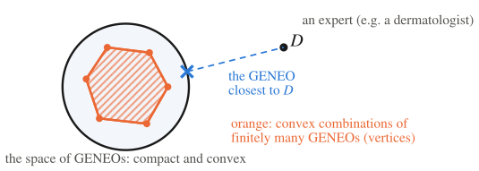
Why we care: suppose an expert $D$ (e.g. a dermatologist classifying skin lesions) is the observer we want to imitate. Inside the compact and convex space of GENEOs we can look for the GENEO closest to $D$, e.g. by optimising over convex combinations of a finite set of GENEOs. The problem is well posed: compactness gives existence and finite approximations, convexity gives a nice search space.

“GENEOs looking at GENEOs”: an observer $F$ is itself an object that other operators can observe and compare.

Comparing data through GENEOs and persistence

Let ${\phi }_1,{\phi }_2\in \Phi$ and let $\mathcal{F}$ be a set of GENEOs (a set of observers).

Definition – Pseudo-metrics induced by a family of GENEOs

$$D_{\mathcal{F},\Phi }({\phi }_1,{\phi }_2)=\underset{F\in \mathcal{F}}{\sup }\Vert F({\phi }_1)-F({\phi }_2){\Vert }_{\infty },$$ $$D_{\mathrm{match}}^{\mathcal{F},k}({\phi }_1,{\phi }_2)=\underset{F\in \mathcal{F}}{\sup }{d}_{\mathrm{match}}\left({\mathrm{Dgm}}_k\right(F({\phi }_1)),{\mathrm{Dgm}}_k(F({\phi }_2)\left)\right).$$

In the second one, each observer $F$ first transforms the data, then we compare the persistence diagrams (in degree $k$) of the results.

Stability

$$D_{\mathrm{match}}^{\mathcal{F},k}({\phi }_1,{\phi }_2)\le D_{\mathcal{F},\Phi }({\phi }_1,{\phi }_2)\le \Vert {\phi }_1-{\phi }_2{\Vert }_{\infty },$$

by the stability theorem of persistence and the non-expansivity of each $F$. Moreover $D_{\mathrm{match}}^{\mathcal{F},k}\le d_G$.

The invariance of $D_{\mathrm{match}}^{\mathcal{F},k}$ is decided by the chosen operators $\mathcal{F}$. Persistent homology alone is invariant under every isomorphism (Lecture 6), which is often too much. Composing with $T$-equivariant GENEOs we get a pseudo-metric that is strongly $G$-invariant, $D_{\mathrm{match}}^{\mathcal{F},k}({\phi }_1\circ g,{\phi }_2)=D_{\mathrm{match}}^{\mathcal{F},k}({\phi }_1,{\phi }_2\circ g)=D_{\mathrm{match}}^{\mathcal{F},k}({\phi }_1,{\phi }_2)$ for $g\in G$, but is no longer forced to ignore every other isomorphism: how much it sees depends on the choice of $\mathcal{F}$. And it is still cheap to compute (finitely many bottleneck distances).

Extra: GENEOs + persistence recover the natural pseudo-distance

From Frosini et al. (Ch. 5, Theorem 15 and Corollary 13): under mild assumptions on $\Phi$ (non-negative functions, $\Phi$ containing the needed constant functions, and $H_k$ of the domain non-zero), if $\mathcal{F}$ is the set of all GENEOs from $(\Phi ,G)$ to itself (with $T=\mathrm{id}$), then

$$D_{\mathrm{match}}^{\mathcal{F},k}=d_G,$$

and by compactness a finite set of GENEOs approximates $d_G$ within any $\epsilon >0$. So the natural pseudo-distance, the “ground truth” that is hard to compute directly, can be approximated by persistence diagrams of data seen through finitely many GENEOs.

Recap

• Perception pair $(\Phi ,G)$ = the observer: measurements plus equivalences. Every $g\in {\mathrm{Iso}}_{\Phi }(K)$ is a $D_V$-isometry (Prop. 41); if $D_V$ is a metric, so is $D_G$.
• GEO: $F(\phi \circ g)=F(\phi )\circ T(g)$ with $T$ a homomorphism. GENEO: in addition $\Vert F({\phi }_1)-F({\phi }_2){\Vert }_{\infty }\le \Vert {\phi }_1-{\phi }_2{\Vert }_{\infty }$.
• Trivial $T$ gives invariant operators (e.g. persistence diagrams).
• GENEOs are non-expansive for natural pseudo-distances: $d_H(F{\phi }_1,F{\phi }_2)\le d_G({\phi }_1,{\phi }_2)$.
• $\Phi ,\Psi$ compact $\Rightarrow$ the space of GENEOs is compact. Combinations with $\sum |a_i|\le 1$ are GENEOs, and $\Psi$ convex $\Rightarrow$ the space is convex.
• $D_{\mathrm{match}}^{\mathcal{F},k}\le D_{\mathcal{F},\Phi }\le \Vert \cdot {\Vert }_{\infty }$ and $D_{\mathrm{match}}^{\mathcal{F},k}\le d_G$, with equality when $\mathcal{F}$ contains all GENEOs.

References

• M. G. Bergomi, P. Frosini, D. Giorgi, N. Quercioli, Towards a topological–geometrical theory of group equivariant non-expansive operators for data analysis and machine learning, Nature Machine Intelligence 1 (2019), 423–433, arXiv:1812.11832.
• P. Frosini, U. Fugacci, N. Quercioli, F. Tombari, Persistent Homology and Equivariance in Data Analysis: A Topological Introduction, arXiv:2606.21084 (2026), Ch. 5: perception pairs, natural pseudo-distance, GENEOs, compactness and convexity, persistence-induced pseudo-metrics.

---

Handwritten source: tdafull.pdf, page 7