2025.01.20 - Lecture 6

← Lecture 5 · Lecture 7 →

In this lecture (20 January)

• A basis for the persistent homology group
• Properties of persistent Betti number functions
• Multiplicity and discontinuities of the persistent Betti numbers
• Persistence diagrams and the representation theorem
• Matching (bottleneck) distance, stability theorem, Wasserstein distances

Recall from Lecture 5: for $u\le v$ the inclusion $K_u^{\phi }\subseteq K_v^{\phi }$ induces

$$i_{u,v}^{\ast }:H_p(K_u^{\phi })⟶H_p(K_v^{\phi }),$$

with $i_{u,u}^{\ast }=\mathrm{id}$ (identity) and $i_{u,w}^{\ast }=i_{v,w}^{\ast }\circ i_{u,v}^{\ast }$ (functoriality), and

$$H_p^{\phi }(u,v):=\mathrm{Im}{i}_{u,v}^{\ast }\subseteq H_p(K_v^{\phi }),{\beta }_p^{\phi }(u,v)=\dim H_p^{\phi }(u,v).$$

A basis for the persistent homology group

Take $p$-cycles $z_1,\dots ,z_h\in C_p(K_u^{\phi })$ such that $\{[z_1{]}_u,\dots ,[z_h{]}_u\}$ is a basis of $H_p(K_u^{\phi })$, where $[\cdot {]}_u$ is the class in $K_u^{\phi }$.

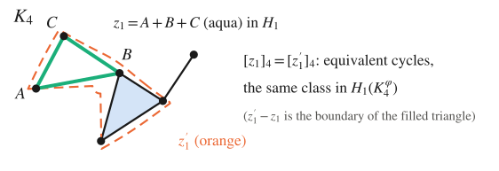
In $K_4$ (the sublevel complex at level 4), $z_1$ is the cycle through $A,B,C$ (aqua). The orange cycle $z_1^{\prime }$ goes around the same hole and around the filled triangle, and $[z_1{]}_4=[z_1^{\prime }{]}_4$: they are different cycles representing the same class in $H_1(K_4^{\phi })$, because they differ by the boundary of the filled triangle. So $z_1$ gives a basis vector of $H_1(K_4^{\phi })$.

Now look at the same cycles at a later level $v$, i.e. at the classes $[z_1{]}_v,\dots ,[z_h{]}_v\in H_p(K_v^{\phi })$.

• $\{[z_1{]}_v,\dots ,[z_h{]}_v\}$ spans $\mathrm{Im}{i}_{u,v}^{\ast }=H_p^{\phi }(u,v)$: the images of a basis span the image of a linear map.
• Since $i_{u,v}^{\ast }$ is not injective in general, it is not a basis: some classes may have died ($[z_i{]}_v=0$) and some may have become equal or dependent.
• We can extract a basis $\{[z_{i_1}{]}_v,\dots ,[z_{i_k}{]}_v\}$ of $H_p^{\phi }(u,v)$: these are the holes already present at level $u$ that are still alive at level $v$.

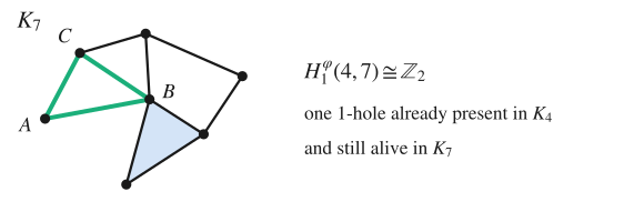
At level $7$ new simplices have entered, but the hole $ABC$ is still there: $H_1^{\phi }(4,7)\cong {\mathbb{Z}}_2$, one hole already present in $K_4$ and still alive in $K_7$.

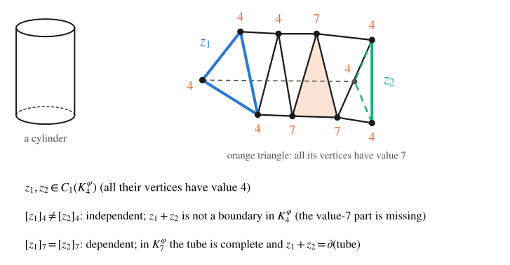
Two classes that merge. $z_1,z_2\in C_1(K_4^{\phi })$ are the two end loops of a triangulated tube, like the two circles of a cylinder (dashed edges are at the back); the numbers are the values of the vertices. At level 4 the tube is not complete (the vertices with value 7, like those of the orange triangle, have not entered yet), so $z_1+z_2$ is not the boundary of any chain and $[z_1{]}_4\ne [z_2{]}_4$: the classes are independent. At level 7 the missing simplices enter, the tube is complete and $z_1+z_2=\partial (\text{tube})$, so $[z_1{]}_7=[z_2{]}_7$: the classes are dependent. The images of the two basis vectors are no longer a basis: $H_1^{\phi }(4,7)$ has dimension 1 (if there are no other holes).

Properties of persistent Betti number functions

Properties of ${\beta }_p^{\phi }(u,v)$ (for $u<v$)

1. Right-continuity in both variables: for every $(u,v)$ and every $\epsilon >0$ small enough,

$${\beta }_p^{\phi }(u,v)={\beta }_p^{\phi }(u+\epsilon ,v)={\beta }_p^{\phi }(u,v+\epsilon )={\beta }_p^{\phi }(u+\epsilon ,v+\epsilon ).$$

2. Monotonicity: ${\beta }_p^{\phi }(u,v)$ is non-decreasing in $u$ and non-increasing in $v$.
3. Invariance under isomorphisms: ${\beta }_p^{\phi }={\beta }_p^{\phi \circ g^{-1}}$ for every isomorphism $g$ (in particular for every $g\in {\mathrm{Iso}}_{\Phi }(K)$).

Why 1. $K$ is finite and $\phi$ takes finitely many values. Sublevel sets are defined with "$\le$", so $K_{u+\epsilon }^{\phi }=K_u^{\phi }$ as long as no value of $\phi$ lies in $(u,u+\epsilon ]$. Nothing changes immediately to the right of $u$.

Why 2. If $u\le u^{\prime }<v$, then $i_{u,v}^{\ast }=i_{u^{\prime },v}^{\ast }\circ i_{u,u^{\prime }}^{\ast }$, so $\mathrm{Im}{i}_{u,v}^{\ast }\subseteq \mathrm{Im}{i}_{u^{\prime },v}^{\ast }$ and $\beta (u,v)\le \beta (u^{\prime },v)$: waiting longer before starting to count, we see more holes. If $u<v\le v^{\prime }$, then $i_{u,v^{\prime }}^{\ast }=i_{v,v^{\prime }}^{\ast }\circ i_{u,v}^{\ast }$, and composing with another map cannot increase the rank, so $\beta (u,v^{\prime })\le \beta (u,v)$: asking holes to survive longer, we see fewer.

Why 3. An isomorphism just renames the vertices. It maps the sublevel complexes of $\phi$ onto those of $\phi \circ g^{-1}$, hence their homology groups isomorphically, so ${\beta }_p$ does not change.

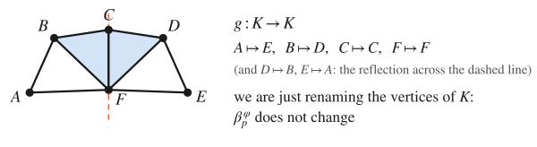
Here $g:K\to K$ with $A\mapsto E$, $B\mapsto D$, $F\mapsto F$, $C\mapsto C$ (a reflection of the complex): we are just renaming the vertices of $K$, and ${\beta }_p^{\phi }$ does not change.

Consequence: persistence cannot see the group

Property 3 says that persistent homology is invariant under every isomorphism: it cannot distinguish $\phi$ from $\phi \circ g$. This is good if we want invariance, but it is often too much invariance, since it ignores how the data are transformed. GENEOs (Lecture 7) are the tool to tune it.

Multiplicity

Definition – Multiplicity of a box

For $u<v$ and $\epsilon ,\eta >0$ with $u+\epsilon <v-\eta$:

$${\mu }_{\epsilon ,\eta }^{\phi }(u,v)={\beta }_p^{\phi }(u+\epsilon ,v-\eta )-{\beta }_p^{\phi }(u-\epsilon ,v-\eta )-{\beta }_p^{\phi }(u+\epsilon ,v+\eta )+{\beta }_p^{\phi }(u-\epsilon ,v+\eta ),$$

an alternating sum of the values of ${\beta }_p^{\phi }$ at the four corners of the rectangle $[u-\epsilon ,u+\epsilon ]\times [v-\eta ,v+\eta ]$ (plus at the bottom-right and top-left corners, minus at the other two).

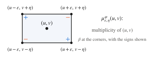
Meaning. ${\beta }_p^{\phi }(a,b)$ counts the features (holes) born at or before $a$ and still alive at $b$. Then $\beta (u+\epsilon ,v-\eta )-\beta (u-\epsilon ,v-\eta )$ counts the features born in $(u-\epsilon ,u+\epsilon ]$ that are alive at $v-\eta$, and $\beta (u+\epsilon ,v+\eta )-\beta (u-\epsilon ,v+\eta )$ counts those still alive at $v+\eta$. The difference counts the features

$$\text{born in }(u-\epsilon ,u+\epsilon ]\text{and dead in }(v-\eta ,v+\eta ].$$

Hence:

• ${\mu }_{\epsilon ,\eta }(u,v)\ge 0$;
• enlarging the rectangle can only add features: ${\mu }_{{\epsilon }^{\prime },{\eta }^{\prime }}(u,v)\ge {\mu }_{\epsilon ,\eta }(u,v)$ for ${\epsilon }^{\prime }\ge \epsilon$, ${\eta }^{\prime }\ge \eta$.

Definition – Multiplicity of a point

• For $u<v$ (a proper point): ${\mu }^{\phi }(u,v)={\lim }_{\epsilon \to 0^{+}}{\mu }_{\epsilon ,\epsilon }^{\phi }(u,v)$, which exists by monotonicity. It is the number of features born exactly at $u$ and dying exactly at $v$.
• For a point at infinity $(u,\infty )$: ${\nu }^{\phi }(u)={\lim }_{\epsilon \to 0^{+}}({\beta }_p^{\phi }(u+\epsilon ,v)-{\beta }_p^{\phi }(u-\epsilon ,v))$ with $v>\max \phi$: the number of features born at $u$ that never die.

Discontinuities of the persistent Betti numbers

Take the function of Lecture 1 ($\phi (0)=0.2$, $\phi (0.2)=0.6$, $\phi (0.4)=0.4$, $\phi (0.6)=1$, $\phi (1)=0$) and draw ${\beta }_0^{\phi }(u,v)$ on the half-plane $\{u<v\}$:

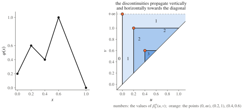
• $u<0$: nothing is born yet, $\beta =0$;
• $0\le u<0.2$: only the component born at $0$, which never dies: $\beta =1$;
• $0.2\le u<0.4$: $\beta =2$ if $v<1$ (the component born at $0.2$ dies at $1$), otherwise $\beta =1$;
• $0.4\le u$: $\beta =3$ if $v<0.6$, $\beta =2$ if $0.6\le v<1$, $\beta =1$ if $v\ge 1$.

Each pair $(a,b)$ of the diagram contributes $+1$ on the triangle $\{a\le u<v<b\}$, and $\beta$ is the number of triangles superimposed at $(u,v)$. The pair $(0,\infty )$ contributes on the whole region $u\ge 0$, $(0.2,1)$ on the triangle $\{0.2\le u<v<1\}$, $(0.4,0.6)$ on the small triangle $\{0.4\le u<v<0.6\}$. In the figure, darker blue means a larger $\beta$, and the numbers are the values of ${\beta }_0^{\phi }$.

Discontinuities propagate vertically and horizontally towards the diagonal

The discontinuity lines of ${\beta }_p^{\phi }$ are vertical and horizontal segments: from each point $(a,b)$ of the diagram, a vertical segment goes down to the diagonal and a horizontal segment goes right to the diagonal. The points of the diagram are the corners where a vertical and a horizontal discontinuity line meet.

Persistence diagrams

Definition – Persistence diagram

The persistence diagram ${\mathrm{Dgm}}_p(\phi )$ is the multiset containing

• every point $(u,v)$ with $u<v$ and ${\mu }^{\phi }(u,v)={\lim }_{\epsilon \to 0^{+}}{\mu }_{\epsilon ,\epsilon }^{\phi }(u,v)>0$, counted ${\mu }^{\phi }(u,v)$ times (proper cornerpoints);
• every point $(u,\infty )$ with ${\nu }^{\phi }(u)>0$, counted ${\nu }^{\phi }(u)$ times (cornerpoints at infinity);
• the diagonal $\Delta$, counted infinitely many times.

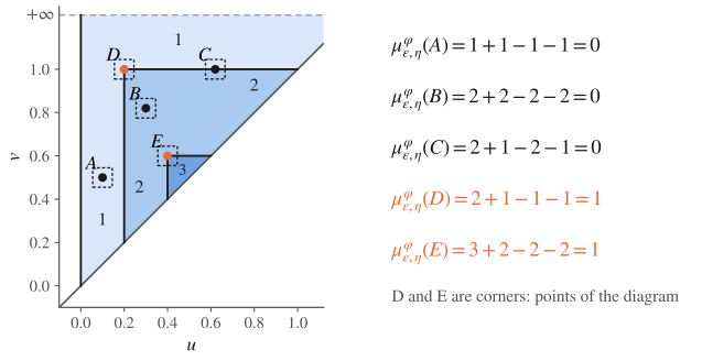
How to read the example (the numbers are the values of $\beta$ in the regions):

• $\mu (A)=1+1-1-1=0$ and $\mu (B)=2+2-2-2=0$: $A$ and $B$ lie inside regions where $\beta$ is constant, so the four corners cancel;
• $\mu (C)=2+1-2-1=0$: $C$ lies on a single (horizontal) discontinuity line, and the corners cancel in pairs;
• $\mu (D)=2+1-1-1=1$ and $\mu (E)=3+2-2-2=1$: $D$ and $E$ are corners, where a vertical and a horizontal discontinuity meet.

So $D$ and $E$ are the points of the diagram.

Representation Theorem: persistence diagram $⟺\beta$

The diagram determines the persistent Betti numbers and vice versa:

$${\beta }_p^{\phi }(\bar{u},\bar{v})=\sum _{\begin{array}{c}u\le \bar{u}\\ v>\bar{v}\end{array}}{\mu }^{\phi }(u,v)+\sum _{u\le \bar{u}}{\nu }^{\phi }(u),$$

i.e. ${\beta }_p^{\phi }(\bar{u},\bar{v})$ is the number of points of ${\mathrm{Dgm}}_p(\phi )$ (with multiplicity) in the upper-left quadrant $\{u\le \bar{u},v>\bar{v}\}$. This is the “superimposed triangles” picture above. The diagram is a compact encoding of the whole function ${\beta }_p^{\phi }$. (See Frosini et al., Theorem 4.)

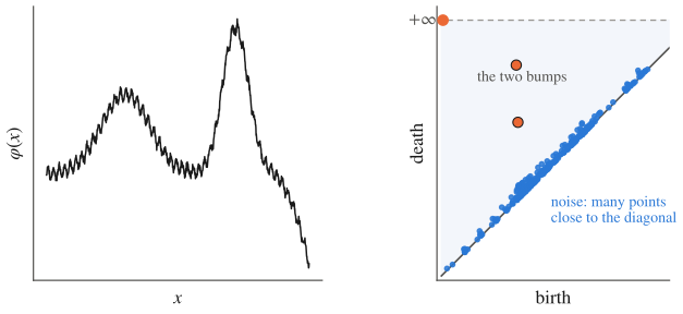
Example: a noisy function. The two main bumps give two points far from the diagonal (plus the point at infinity), while the noise gives many points close to the diagonal.

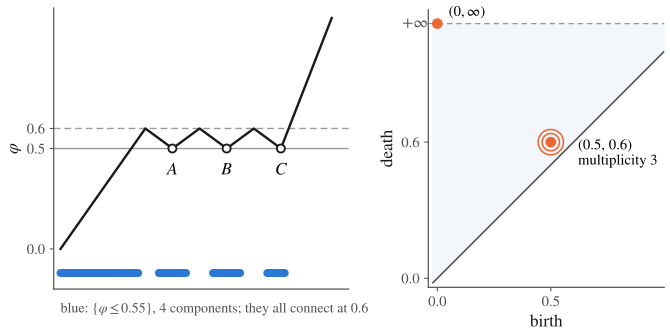
Example: a point with multiplicity 3. After the global minimum at height $0$, the function has three local minima $A,B,C$ at height $0.5$, separated by local maxima at height $0.6$. Each of $A,B,C$ starts a component at $0.5$, and all three merge with the older component at $0.6$. The diagram has $(0,\infty )$ and the point $(0.5,0.6)$ with multiplicity 3 (drawn with concentric circles).

Matching distance

How do we compare two persistence diagrams? We match their points: a bijection between $\mathrm{Dgm}(\phi )$ and $\mathrm{Dgm}(\psi )$, where a point may also be matched to the diagonal $\Delta$ (which has infinitely many copies, so the two diagrams always have “the same number of points”).

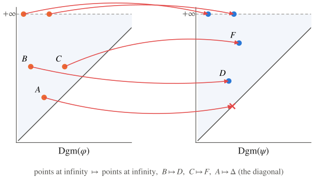
$\mathrm{Dgm}(\phi )=\{(u_1,\infty ),(u_2,\infty ),A,B,C,\Delta ,\dots \}$ and $\mathrm{Dgm}(\psi )=\{({\bar{u}}_1,\infty ),({\bar{u}}_2,\infty ),D,F,\Delta ,\dots \}$. Points at infinity are matched among themselves, $B\mapsto D$, $C\mapsto F$, and $A\mapsto \Delta$: $A$ is the point closest to the diagonal, and it is matched with “nothing”.

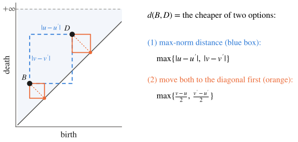
Cost of matching two points. For $P=(u,v)$ and $P^{\prime }=(u^{\prime },v^{\prime })$ there are two options: move $P$ directly onto $P^{\prime }$ (max-norm distance), or send both to the diagonal. Their cost is

$$d(P,P^{\prime })=\min \{\max \{|u-u^{\prime }|,|v-v^{\prime }|\},\max \{\frac{v-u}{2},\frac{v^{\prime }-u^{\prime }}{2}\left\}\right\},d(P,\Delta )=\frac{v-u}{2},$$

$d((u,\infty ),(u^{\prime },\infty ))=|u-u^{\prime }|$, and $d(\Delta ,\Delta )=0$. $(v-u)/2$ is the max-norm distance from $(u,v)$ to the closest point of the diagonal, so points with little persistence are cheap to delete.

Definition – Matching (bottleneck) distance

For every bijection $f:\mathrm{Dgm}(\phi )\to \mathrm{Dgm}(\psi )$ define $\mathrm{cost}(f)={\max }_{P\in \mathrm{Dgm}(\phi )}d(P,f(P))$. Then

$$d_{\mathrm{match}}(\mathrm{Dgm}(\phi ),\mathrm{Dgm}(\psi ))=\underset{f}{\inf }\mathrm{cost}(f).$$

It is a metric on persistence diagrams, also called the bottleneck distance: only the worst-matched pair counts.

Example

$\phi$ is the function of Lecture 1, ${\mathrm{Dgm}}_0(\phi )=\{(0,\infty ),(0.2,1),(0.4,0.6)\}$. $\psi$ is the same function with the small bump removed and a lower maximum: $\psi (0)=0.2$, $\psi (0.2)=0.6$, $\psi (0.4)=0.6$, $\psi (0.6)=0.9$, $\psi (1)=0$. Then ${\mathrm{Dgm}}_0(\psi )=\{(0,\infty ),(0.2,0.9)\}$.

• Matching $(0,\infty )\mapsto (0,\infty )$ (cost $0$), $(0.2,1)\mapsto (0.2,0.9)$ (cost $0.1$), $(0.4,0.6)\mapsto \Delta$ (cost $0.2/2=0.1$) has cost $0.1$.
• Matching instead $(0.4,0.6)\mapsto (0.2,0.9)$ costs $\min \{\max (0.2,0.3),\max (0.1,0.35)\}=0.3$, and then $(0.2,1)\mapsto \Delta$ costs $0.4$. Worse.

$(0.4,0.6)$ must go either to $\Delta$ (cost $0.1$) or to $(0.2,0.9)$ (cost $0.3$), so no matching costs less than $0.1$, and $d_{\mathrm{match}}=0.1$. Compare with $\Vert \phi -\psi {\Vert }_{\infty }=0.2$ (at $x=0.4$): consistent with the stability theorem below.

Stability

Stability Theorem

For $\phi ,\psi \in \Phi$ and every degree $p$:

$$d_{\mathrm{match}}({\mathrm{Dgm}}_p(\phi ),{\mathrm{Dgm}}_p(\psi ))\le \Vert \phi -\psi {\Vert }_{\infty },$$

and, since diagrams do not see isomorphisms (${\mathrm{Dgm}}_p(\psi \circ g)={\mathrm{Dgm}}_p(\psi )$, property 3),

$$d_{\mathrm{match}}({\mathrm{Dgm}}_p(\phi ),{\mathrm{Dgm}}_p(\psi ))\le \underset{g\in G}{\min }\Vert \phi -\psi \circ g{\Vert }_{\infty }=d_G(\phi ,\psi ).$$

Meaning:

• Robustness to noise: a small perturbation of the data (small $\Vert \phi -\psi {\Vert }_{\infty }$) moves the diagram only a little. Noise creates points close to the diagonal, which are cheap to match to $\Delta$.
• A computable lower bound for the natural pseudo-distance. $d_G$ is difficult to compute (it is a minimisation over the group), while diagrams and $d_{\mathrm{match}}$ are computable. If the diagrams are far apart, the data are certainly far apart up to $G$. The converse is false: different data can have the same diagram.

Wasserstein distances

Definition – $q$-th Wasserstein distance

For two persistence diagrams $X,Y$ and $q\ge 1$:

$$W_q(X,Y)=[\underset{\eta :X\to Y}{\inf }\sum _{x\in X}\Vert x-\eta (x){\Vert }_{\infty }^q{]}^{1/q},$$

where $\eta$ ranges over the bijections (points may be matched to the diagonal, at cost equal to their distance from it). The bottleneck distance is the case $q=\infty$:

$$W_{\infty }(X,Y)=\underset{\eta :X\to Y}{\inf }\underset{x\in X}{\sup }\Vert x-\eta (x){\Vert }_{\infty }.$$

$W_q$ adds up all the displacements, so it is sensitive to many small differences, e.g. a lot of noise points. The bottleneck distance only looks at the largest displacement. (The handwritten notes omit the exponent $1/q$.)

Recap

• From a basis $\{[z_i{]}_u\}$ of $H_p(K_u)$ we get a spanning set $\{[z_i{]}_v\}$ of $H_p^{\phi }(u,v)$, not a basis, because $i_{u,v}^{\ast }$ is not injective.
• ${\beta }_p^{\phi }$ is right-continuous, non-decreasing in $u$, non-increasing in $v$, and invariant under isomorphisms.
• ${\mu }_{\epsilon ,\eta }(u,v)$ (alternating sum at the corners of a box) counts the features born near $u$ and dying near $v$. Points with $\mu >0$ form the persistence diagram.
• Representation theorem: ${\beta }_p^{\phi }(\bar{u},\bar{v})$ is the number of diagram points with $u\le \bar{u}$, $v>\bar{v}$.
• $d_{\mathrm{match}}$ = best bijection (diagonal allowed), cost = worst pair. Stability: $d_{\mathrm{match}}\le d_G\le \Vert \phi -\psi {\Vert }_{\infty }$.
• $W_q$ sums the costs; $W_{\infty }$ is the bottleneck distance.

References

• P. Frosini, U. Fugacci, N. Quercioli, F. Tombari, Persistent Homology and Equivariance in Data Analysis: A Topological Introduction, arXiv:2606.21084 (2026), Ch. 3: persistent Betti numbers functions, multiplicity, representation theorem, matching distance and its stability.

---

Handwritten source: tdafull.pdf, page 6