2025.01.18 - Lecture 5

← Lecture 4 · Lecture 6 →

In this lecture (17 January in the handwritten notes)

• The setting: functions on $K$, isomorphisms, ${\mathrm{Iso}}_{\Phi }(K)$, simplicial perception pairs
• Three pseudo-metrics: $D_V$, $D_G$, $D_{\Phi }$
• The natural pseudo-distance $d_G$ and its properties
• Choosing the level of analysis: a first look at a persistence diagram
• Sublevel complexes and filtrations
• Persistence modules, persistent homology groups, persistent Betti numbers

What we need for the natural pseudo-distance

Four ingredients.

① Functions on a complex. A geometric simplicial complex $K$ and functions ${\phi }^{\prime }:\mathrm{Vert}(K)\to \mathbb{R}$, extended to $\phi :K\to \mathbb{R}$ by

$$\phi (⟨u_0,\dots ,u_k⟩)=\max ({\phi }^{\prime }(u_0),\dots ,{\phi }^{\prime }(u_k))$$

(see Lecture 4). E.g. a triangle with ${\phi }^{\prime }(A)=1$, ${\phi }^{\prime }(B)={\phi }^{\prime }(C)=2$ gets $\phi (\alpha )=2$. The set $\Phi$ of these functions is our set of measurements: $\phi \in \Phi$.

② The isomorphisms of $K$. $\mathrm{Iso}(K)$ is the set of bijections $f:\mathrm{Vert}(K)\to \mathrm{Vert}(K)$ with

$$⟨u_0,\dots ,u_k⟩\in K⟺⟨f(u_0),\dots ,f(u_k)⟩\in K.$$

③ The isomorphisms that preserve the measurements. ${\mathrm{Iso}}_{\Phi }(K)\subseteq \mathrm{Iso}(K)$ is the set of $g$ such that $\phi \circ g\in \Phi$ and $\phi \circ g^{-1}\in \Phi$ for every $\phi \in \Phi$. It is a group.

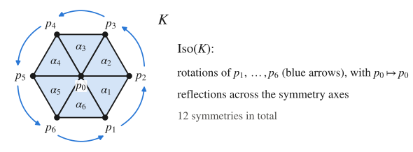
Example – the hexagon

$K$ is a hexagon triangulated from its centre $p_0$, with boundary vertices $p_1,\dots ,p_6$ and triangles ${\alpha }_1,\dots ,{\alpha }_6$. $\mathrm{Iso}(K)$ consists of the 12 symmetries of the hexagon: the rotations of $p_1,\dots ,p_6$ and the reflections across its symmetry axes. They all fix the centre ($p_0\mapsto p_0$), the only vertex belonging to 6 edges.

Whether a symmetry belongs to ${\mathrm{Iso}}_{\Phi }(K)$ depends on $\Phi$:

• if $\Phi$ contains only the function with ${\phi }^{\prime }(p_1)=\cdots ={\phi }^{\prime }(p_6)=1$ and ${\phi }^{\prime }(p_0)=2$, every symmetry leaves it unchanged, so ${\mathrm{Iso}}_{\Phi }(K)=\mathrm{Iso}(K)$;
• if $\Phi$ contains only a function with different values $1,2,\dots ,6$ on $p_1,\dots ,p_6$, every non-trivial symmetry changes it into a function that is not in $\Phi$, so ${\mathrm{Iso}}_{\Phi }(K)=\{\mathrm{id}\}\ne \mathrm{Iso}(K)$.

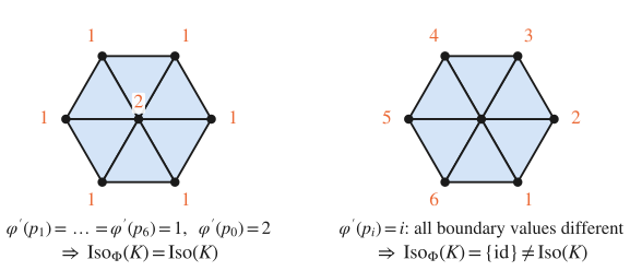
If $\Phi ={\mathbb{R}}^{\mathrm{Vert}(K)}$ (all possible functions on the vertices), every isomorphism preserves $\Phi$ and ${\mathrm{Iso}}_{\Phi }(K)=\mathrm{Iso}(K)$. The smaller (more structured) $\Phi$ is, the fewer isomorphisms survive. $\Phi$ describes the observer.

④ The group we work with.

Definition – Simplicial perception pair

A pair $(\Phi ,G)$ where $\Phi$ is a set of functions on $K$ (built as in ①) and $G\subseteq {\mathrm{Iso}}_{\Phi }(K)$ is a subgroup is a (simplicial) perception pair. For every $\phi \in \Phi$ and $g\in G$ we have $\phi \circ g\in \Phi$ and $\phi \circ g^{-1}\in \Phi$.

$G$ contains the transformations we want to consider irrelevant (rotations, renamings, …), and we can choose it smaller than ${\mathrm{Iso}}_{\Phi }(K)$.

Three pseudo-metrics

Let $V=\mathrm{Vert}(K)$. Everything is measured through the instruments $\Phi$, not with the Euclidean metric of the space where $K$ is drawn.

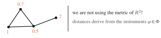
Definition – $D_V$, $D_G$, $D_{\Phi }$

1. On the vertices (distance between points):

$$D_V(v_1,v_2)=\underset{\phi \in \Phi }{\sup }|\phi (v_1)-\phi (v_2)|.$$

Two vertices are far apart iff some measurement distinguishes them well.
2. On the group $G\subseteq {\mathrm{Iso}}_{\Phi }(K)$ (distance between transformations):

$$D_G(g_1,g_2)=\underset{\phi \in \Phi }{\sup }\Vert \phi \circ g_1-\phi \circ g_2{\Vert }_{\infty }.$$

3. On the space of signals $\Phi$:

$$D_{\Phi }({\phi }_1,{\phi }_2)=\Vert {\phi }_1-{\phi }_2{\Vert }_{\infty }=\underset{v\in V}{\max }|{\phi }_1(v)-{\phi }_2(v)|.$$

• They are pseudo-metrics: $D_V(v_1,v_2)=0$ if no instrument can tell $v_1$ and $v_2$ apart, even when $v_1\ne v_2$.
• In 3, taking the max over the vertices or over all simplices gives the same value: $|{\max }_i{\phi }_1(u_i)-{\max }_i{\phi }_2(u_i)|\le {\max }_i|{\phi }_1(u_i)-{\phi }_2(u_i)|$, and vertices are simplices.
• The action of any $G\subseteq {\mathrm{Iso}}_{\Phi }(K)$ preserves all three: $D_{\Phi }({\phi }_1\circ g,{\phi }_2\circ g)=D_{\Phi }({\phi }_1,{\phi }_2)$ (composing with a bijection of the vertices only reorders the values), $D_V(g(v_1),g(v_2))=D_V(v_1,v_2)$ (proved in Lecture 7), and $D_G(g\circ g_1,g\circ g_2)=D_G(g_1\circ g,g_2\circ g)=D_G(g_1,g_2)$. The key fact is that $\phi \mapsto \phi \circ g$ is a bijection of $\Phi$ onto itself.

The natural pseudo-distance

We do not want to compare $\phi$ and $\psi$ as they are, but up to the transformations in $G$: try every alignment of $\psi$ and keep the best.

Definition – Natural pseudo-distance

For a perception pair $(\Phi ,G)$ and $\phi ,\psi \in \Phi$:

$$d_G(\phi ,\psi )=\underset{g\in G}{\min }\Vert \phi -\psi \circ g{\Vert }_{\infty }.$$

(Here $G$ is finite, so the minimum exists; in general it is an infimum.)

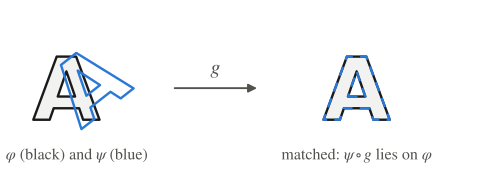
Two copies of the letter A, one of them rotated: their sup-distance is large, but after applying the right rotation they match, so $d_G$ is small (zero if they are identical up to rotation).

Proposition – $d_G$ is a pseudo-metric

For all $\phi ,\psi ,\chi \in \Phi$: $d_G(\phi ,\phi )=0$, $d_G(\phi ,\psi )=d_G(\psi ,\phi )$ and $d_G(\phi ,\psi )\le d_G(\phi ,\chi )+d_G(\chi ,\psi )$.

Proof

We use two facts: $\Vert \alpha \circ h-\beta \circ h{\Vert }_{\infty }=\Vert \alpha -\beta {\Vert }_{\infty }$ for any bijection $h$ (composing with a bijection only reorders the values), and $g\mapsto g^{-1}$ is a bijection of $G$.

• $d_G(\phi ,\phi )\le \Vert \phi -\phi \circ \mathrm{id}{\Vert }_{\infty }=0$.
• Symmetry:

$$d_G(\phi ,\psi )=\underset{g\in G}{\min }\Vert \phi -\psi \circ g{\Vert }_{\infty }=\underset{g\in G}{\min }\Vert \phi \circ g^{-1}-\psi {\Vert }_{\infty }=\underset{g^{-1}\in G}{\min }\Vert \psi -\phi \circ g^{-1}{\Vert }_{\infty }=d_G(\psi ,\phi ).$$

• Triangle inequality: for every $f,g\in G$,

$$\Vert \phi -\psi \circ g\circ f{\Vert }_{\infty }\le \Vert \phi -\chi \circ f{\Vert }_{\infty }+\Vert \chi \circ f-\psi \circ g\circ f{\Vert }_{\infty }=\Vert \phi -\chi \circ f{\Vert }_{\infty }+\Vert \chi -\psi \circ g{\Vert }_{\infty }.$$

Minimise over $g$ (as $g$ varies, $g\circ f$ covers all of $G$) and then over $f$.

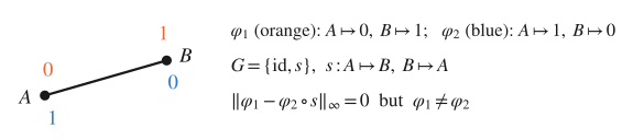
Example – distance zero between different functions

$K$ is a segment $AB$, $G=\{\mathrm{id},s\}$ with $s$ swapping $A$ and $B$. Let ${\phi }_1(A)=0$, ${\phi }_1(B)=1$ and ${\phi }_2(A)=1$, ${\phi }_2(B)=0$. Then ${\phi }_2\circ s={\phi }_1$, so $\Vert {\phi }_1-{\phi }_2\circ s{\Vert }_{\infty }=0$ and $d_G({\phi }_1,{\phi }_2)=0$, although ${\phi }_1\ne {\phi }_2$. So $d_G$ is a pseudo-metric, not a metric.

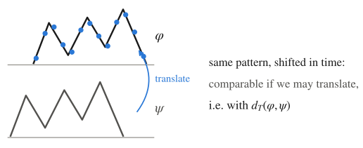
It is very useful for time series: two signals with the same pattern, one shifted in time, are far in the sup-norm but close for $d_T$, where $T$ is a group of time translations.

Properties of $d_G$

1. Enlarging the group does not increase the distance: if $G_1\subseteq G_2$ then

$$d_{G_2}(\phi ,\psi )\le d_{G_1}(\phi ,\psi )\le \Vert \phi -\psi {\Vert }_{\infty },$$

where the last term is $d_{\{\mathrm{id}\}}$. A bigger group gives more ways to align the data. Going from $\{\mathrm{id}\}$ to ${\mathrm{Iso}}_{\Phi }(K)$, the distance can only decrease.
2. Strong invariance: for all $g_1,g_2\in G$,

$$d_G(\phi \circ g_1,\psi \circ g_2)=d_G(\phi ,\psi ).$$

Proof: $\Vert \phi \circ g_1-\psi \circ g_2\circ g{\Vert }_{\infty }=\Vert \phi -\psi \circ (g_2\circ g\circ g_1^{-1}){\Vert }_{\infty }$, and $g_2\circ g\circ g_1^{-1}$ ranges over all of $G$ as $g$ does.

$d_G$ is the “ground truth” for comparing data up to $G$, but it is hard to compute: we must optimise over the whole group. Persistent homology gives computable lower bounds for it (Lecture 6).

Choosing the level of analysis

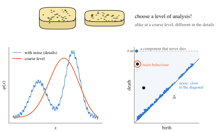
What counts as “the same” depends on the observer and on the level of detail we care about: two sponges look alike at a coarse level and very different in the details. A noisy function (blue) and its coarse, smooth version (orange) differ only in the details.

The persistence diagram on the right is a preview of Lecture 6:

• the diagonal $\Delta$ is treated as a single abstract point with infinite multiplicity (it lets us match a point with “nothing”);
• a point at $+\infty$ (a half-line going to infinity) means a connected component that never dies;
• the circled point, far from the diagonal, describes the main behaviour of the function (the big bump);
• the points close to the diagonal are the small details or noise. The closer a point is to the diagonal, the smaller the detail it describes.

Sublevel complexes and filtrations

Let $\phi :K\to \mathbb{R}$ be the max-extension of some ${\phi }^{\prime }$. For every $u\in \mathbb{R}$:

Definition – Sublevel complex

$$K_u^{\phi }=\{\sigma \in K:\phi (\sigma )\le u\}.$$

It is a subcomplex of $K$: faces have smaller or equal values. If $u\le v$, then $K_u^{\phi }\subseteq K_v^{\phi }$, so the family $\{K_u^{\phi }{\}}_{u\in \mathbb{R}}$ is a filtration of $K$.

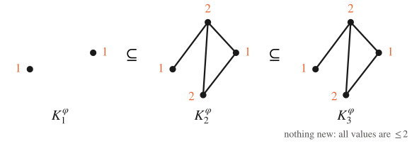
As $u$ grows, simplices enter: first the vertices with small values, then the edges and triangles whose vertices are all present. The sequence of complexes gives a sequence of homology groups $H_p(K_u^{\phi })$, and we want to follow how they change.

Persistence modules and persistent homology groups

Definition – Persistence module

A family of vector spaces $\{V_t{\}}_{t\in \mathbb{R}}$ with linear maps $i_{s,t}:V_s\to V_t$ for $s\le t$ such that

1. functoriality: $i_{r,t}=i_{s,t}\circ i_{r,s}$ for $r\le s\le t$;
2. identity: $i_{t,t}={\mathrm{id}}_{V_t}$.

Our persistence module is $V_t=H_p(K_t^{\phi })$. For $s\le t$ the inclusion $i_{s,t}:K_s^{\phi }\hookrightarrow K_t^{\phi }$ ($K_1\subseteq K_2$) induces a linear map

$$i_{s,t}^{\ast }:H_p(K_s^{\phi })\to H_p(K_t^{\phi }),[z{]}_s\mapsto [z{]}_t,$$

i.e. we take a $p$-cycle $z\in C_p(K_s^{\phi })$ and look at it as a cycle of the bigger complex $K_t^{\phi }$. It is well defined: a cycle is still a cycle in $K_t$, and a boundary is still a boundary. Functoriality holds: $i_{r,t}^{\ast }=i_{s,t}^{\ast }\circ i_{r,s}^{\ast }$.

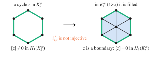
$i_{s,t}^{\ast }$ is in general not injective

A cycle that is a hole in $K_s$ can become a boundary in $K_t$ if the triangles filling it enter between $s$ and $t$. Then $[z{]}_s\ne 0$ but $[z{]}_t=0$.

Definition – Persistent homology group

For $u<v$:

$$H_p^{\phi }(u,v):=\mathrm{Im}{i}_{u,v}^{\ast }\subseteq H_p(K_v^{\phi })$$

is the persistent homology group of $\phi$ computed at $(u,v)$. It contains the $p$-holes that already exist at level $u$ and are still alive at level $v$.

What does it mean? Follow a cycle through the filtration:

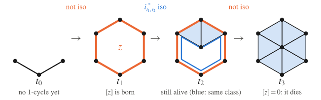
• $t_0$: no cycle yet.
• $t_1$: the homology group changes, a cycle $z$ closes and a class $[z]\in H_1(K_{t_1}^{\phi })$ is born: it is in $H_1(K_{t_1}^{\phi })$ but not in the image of $i_{t_0,t_1}^{\ast }$.
• $t_2$: some triangles enter, but the hole is still there (represented by a different, smaller cycle). $i_{t_1,t_2}^{\ast }$ is an isomorphism on this class.
• $t_3$: the hole is completely filled, $z$ becomes a boundary and the class dies: $[z{]}_{t_3}=0$.

Definition – Persistent Betti number function (rank invariant)

$${\beta }_p^{\phi }(u,v)=\dim H_p^{\phi }(u,v)=\mathrm{rank}{i}_{u,v}^{\ast },u<v,$$

the number of independent $p$-holes born at or before $u$ and still alive at $v$. It is the persistent Betti number function of $\phi$ in degree $p$.

Its properties, and the persistence diagram that summarises it, are the subject of Lecture 6.

Recap

• Simplicial perception pair $(\Phi ,G)$: measurements $\Phi$ on $K$ (max-extensions) and a group $G\subseteq {\mathrm{Iso}}_{\Phi }(K)$ of isomorphisms preserving $\Phi$.
• $D_V$, $D_G$, $D_{\Phi }=\Vert \cdot {\Vert }_{\infty }$: pseudo-metrics defined through the measurements, preserved by $G$.
• $d_G(\phi ,\psi )={\min }_{g\in G}\Vert \phi -\psi \circ g{\Vert }_{\infty }$: a pseudo-metric, non-increasing in $G$, strongly $G$-invariant, hard to compute.
• $K_u^{\phi }=\{\phi \le u\}$ is a filtration. Inclusions induce $i_{u,v}^{\ast }$ on homology, and $H_p^{\phi }(u,v)=\mathrm{Im}{i}_{u,v}^{\ast }$ contains the holes born by $u$ and still alive at $v$. ${\beta }_p^{\phi }(u,v)=\dim H_p^{\phi }(u,v)$.

References

• P. Frosini, U. Fugacci, N. Quercioli, F. Tombari, Persistent Homology and Equivariance in Data Analysis: A Topological Introduction, arXiv:2606.21084 (2026): Ch. 3 (persistent homology groups, persistent Betti numbers) and Ch. 5 (perception pairs, natural pseudo-distance), stated there for continuous functions on topological spaces.

---

Handwritten source: tdafull.pdf, page 5